The Constructible tower
The real and complex numbers can't be constructed. This post builds a replacement that can, and that is exact where they only approximate: the Constructible tower, a tower of finite number systems where every polynomial has its roots, √2 and ∛3 are exact numbers, the imaginary unit appears naturally, and an exact calculus works without limits. With machine-checked proofs in Lean.
Mathematics and physics are written on top of the real numbers \( \mathbb{R} \) and the complex numbers \( \mathbb{C} \), and neither of them can be constructed: almost all of their points have no finite description at all. This post proposes a replacement that can be constructed, and that is exact where \( \mathbb{R} \) only approximates: the Constructible tower, a tower of finite number systems, built one finite step at a time, in which every polynomial finds its roots exactly, where \( i = \sqrt{-1} \) appears naturally as one of its first symbols, and on which an exact calculus works without limits.
Above wallpaper reference1
This post is a follow-up to Infinity is a paradox2, so if you haven't read it, it's worth starting there. It grew out of a constructive discussion on X3 about whether infinity exists, and whether math is invented or discovered. Many thanks to @DoozerDiffuser for pushing back seriously and patiently, forgiving his immature last comment!
As always the ideas are all mine, since current AI/SI models cannot build well-defined abstractions yet. I had this idea at least a year or two! However, I used Opus 5.5 and Fable 5.2.
The reader MUST have incentives to find well-defined abstractions among the chaos, even though what we have here is far from chaos. At least this is how I operate when I read other scientific researches, and I expect my readers to do the same!
The goal, and how this post is organized
The goal is to replace the non-constructible structures \( \mathbb{R} \) and \( \mathbb{C} \) by a constructible one, and to check that what we need from them survives: roots of polynomials, the imaginary unit, rotations, and calculus.
The post has two halves, and the first prepares the second.
The first half is philosophical. It fixes the principles, namely that an object exists when a finite construction produces it, and then answers the objections from the discussion one by one: the infinite set of states, the Axiom of Infinity, the cube, the digits of \( \pi \). Its conclusion is that infinity is a finite rule without a stopping condition, never a finished object. But this leaves a debt. If \( \mathbb{R} \) and \( \mathbb{C} \) aren't constructed, then saying so is not enough: we owe a number system that is constructed and can do their work.
One payment of this debt already exists: constructive analysis, where a real number is a finite rule that produces its digits. It is compatible with the principles of this post, and the post doesn't claim it fails. The second half explores a different and stricter payment, in which not only every number but the number system itself is finite, and every question about its numbers is settled by a finite computation. It argues that this payment is the stronger one. The section "Is the debt already paid?" compares the two.
The second half pays the debt in this stricter way, by construction. It goes in this order:
- Constructible depends on the tools. Straightedge, compass, and origami each solve one more kind of equation, and each gives its own set of numbers over \( \mathbb{Q} \). A short section then asks whether constructive analysis already pays the debt.
- Counting in finite worlds. The Riemann sphere argument of my previous post, redone where every count is honest: bounded rationals, then arithmetic modulo a prime \( p \).
- The Constructible tower. Starting from the integers modulo \( p \), each level adds one new symbol, a root that the previous level lacks. Square roots alone turn out not to be enough, so all radicals are allowed. Whatever root one level misses, a later level adds, and the tower as a whole has every root of every polynomial: its own fundamental theorem of algebra.
- The algebra of the new symbols. A formula tells which symbols are new at each level, and each of them, starting with \( i \), has a conjugation and a norm.
- Calculus without limits. Differences, the fundamental theorem, the chain rule, differential forms, Stokes' theorem, charts, rotations, and the Jacobian, all exact, on every level of the tower.
- Patches with different primes. Charts overlap only on strips, so each patch can carry its own prime. On a strip the calculus stays consistent when both primes exceed the size of the data there, and curvature decides how fast that size grows.
- Levels against iterations. Where \( \mathbb{R} \) reaches \( \sqrt{2} \), \( \sqrt[3]{2} \), or \( \sqrt[3]{3} \) by an iteration that never ends, the tower reaches each of them exactly, in finitely many levels. This is the case that \( \mathbb{CT}_p \) is the stronger number system, together with what becomes of order.
Two remarks on words. Classically, a "constructible number" means one reached by ruler and compass. In this post the Constructible tower, CT for short, is the finite tower of step 3. Like \( \mathbb{R} \) and \( \mathbb{C} \) it gets its own letters: \( \mathbb{CT}_p \) for the tower over the prime \( p \), and \( \mathbb{CT}_{k,p} \) for its level \( k \). The ruler-and-compass tower over \( \mathbb{Q} \), written \( C_k \), is its ancestor: it is the ruler-and-compass row of step 1, and is written out in step 2. And "has every root" is meant in the sense this post defends: every polynomial is solved at a finite level, by a finite construction. The tower as one finished object is never built, and never needed.
Every theorem of the second half is proved in Lean4, a proof checker, so the reader doesn't have to trust the prose. Where a statement is only checked on examples, or argued in words, the text says so.
The conversation in short
The discussion started from a claim by my interlocutor: invention is choosing an arbitrary state from an infinite set of states, discovery is finding the optimal state under a set of constraints, and therefore music is invention, physics is discovery, and math is somewhere in between. I replied that there is no infinite set of states and no platonic universe5 holding them, so math is invention, experimental physics is discovery, and theoretical physics is invention.
From there the objections came in this order:
- I asserted my conclusion without giving definitions.
- The number of possible states is unbounded, and whether that unboundedness is epistemic or ontological is irrelevant.
- Infinite just means unbounded, the same as in the Axiom of Infinity6.
- If infinities don't exist, give an exhaustive list of all the things that can happen today.
- How many squares are in a cube?
- How many digits does \( \pi \) have?
- A rigorous definition of a number that no finite string of digits can represent is a conceptual infinity, and it's real.
- Is infinity being denied conceptually, or only as a physical object?
Along the way, my interlocutor also correctly reminded me that we cannot trisect an angle with ruler and compass. That remark turned out to be more important than it looked, because it touches the Riemann sphere argument of my previous post, so it gets its own section, and it opens the second half of this post.
Objection 1 is fair, so let's start with it.
Principles and definitions
These are the principles I was using in the thread, now written down explicitly.
P1. Existence needs construction. If you claim an object exists, the burden is on you to show it, either by observing it or by constructing it from things that are observed7. This is the constructivist principle8 from my previous post. "You can't prove it doesn't exist" is not evidence that it does.
P2. Every observation is bounded. Every measurement any human has ever made returned a finite number, with finite precision, from a finite apparatus, in a finite time. There is no exception to this in the history of science.
P3. The unbounded comes from recursion. Every "infinite" object in mathematics is introduced by a finite rule that can be applied again to its own output, which is a recursive function9. The rule is finite. What is called "infinite" is the claim that the rule's unfolding exists as a completed whole.
P4. A rule is not its unfolding. A finite rule that contains no stopping condition is still a finite object. Every actual execution of it stops after finitely many steps, because the machine, the paper, the mathematician, or the universe runs out.
Now the definitions:
- An observable is anything we can measure.
- A construction is a finite sequence of applications of finite rules to observables or to previously constructed objects.
- Discovery is finding an object by observation, an object whose existence does not depend on our construction.
- Invention is producing an object by construction.
Under these definitions the conclusion of the thread is no longer an assertion. Every mathematical object we have ever written down, whether a number, a set, or a proof, is the output of a finite construction, so math is invention. Experimental physics measures things that are there whether or not we construct them, so it's discovery. Theoretical physics constructs models, which is invention, and then submits them to discovery through experiment.
Someone may object that once the axioms are fixed, the theorems are already "determined", so proving them is discovery. But "determined" here only means that a finite derivation can be constructed. Until someone constructs it, the theorem is not an object, it's a possibility in our planning, exactly like a melody nobody composed yet. And the axioms and the rules of inference themselves were obviously invented, many times over, in incompatible ways.
Objection: invention is choosing from an infinite set of states
Look at what an inventor actually does. A composer with \( K \) available pitches, writing a melody of \( L \) notes, chooses among at most
\[ K^{L} \]
candidates. With \( K = 88 \) piano keys and \( L = 1000 \) notes, this is an enormous number, but it's a number. Rhythm, dynamics, and timbre each multiply it by another finite factor. No composer ever chose from an infinite set, because no composer ever held one, scanned one, or even described one other than through a finite rule.
More importantly, the "set of all possible melodies" didn't exist before the composer and then get searched. It's a construction we build after the fact to talk about the choice. The composer's real process is a sequence of finitely many local decisions, each among finitely many options. This is the point I was making in the thread when I asked to be shown the infinite set of states being chosen from. Under P1, the burden is on the one who claims the set exists.
So the definition of invention as "choosing from an infinite set" fails twice: the set is not infinite, and it's not chosen from, it's generated.
Objection: infinite just means unbounded, as in the Axiom of Infinity
This is the most important objection, because it rests on a confusion that is more than two thousand years old. Aristotle already separated potential infinity from actual infinity10. Gauss, in an 1831 letter, objected to using an infinite magnitude as a completed thing, accepting infinity only as a manner of speaking about limits. The distinction is precise, and we can write it with quantifiers.
Potential infinity (unboundedness) is a statement about a rule:
\[ \forall n \in \mathbb{N} \quad \exists m \in \mathbb{N} \quad m > n \]
It says: whatever number you have constructed, the successor rule constructs a bigger one. This is a statement about what a finite rule does when applied once more. Notice there's no object here containing all the numbers. Every \( n \) and every \( m \) are single finite constructions.
Actual infinity is what the Axiom of Infinity6 in Zermelo–Fraenkel set theory states:
\[ \exists I \quad \left( \varnothing \in I \ \land \ \forall x \in I \quad x \cup \{x\} \in I \right) \]
It says: there exists a single object \( I \) that already contains the result of every application of the successor rule. This is not "unbounded". This is the claim that the entire unfolding of a recursive rule exists, completed, as one set.
These two statements are not the same, and the difference is exactly the order of the quantifiers. The first one needs only a finite rule. The second one needs an object no one has ever constructed, observed, or could construct, by P2. That's precisely why it has to be postulated as an axiom: in ZF without it, you cannot prove that any infinite set exists. Mathematicians knew it couldn't be constructed, so they assumed it.
So when my interlocutor said infinite means unbounded, "the same definition as used by the Axiom of Infinity", the two halves of that sentence contradict each other. Unbounded is the potential infinity, which I accept as a property of finite rules. The Axiom of Infinity asserts the actual infinity, which is the platonic object I deny.
The Peano axioms11 show the same structure. They give a starting object \( 0 \) and a successor function \( S \). Every natural number anyone has ever used is
\[ S^{k}(0) \quad \text{for some finite } k \]
that is, the output of applying a recursive function a finite number of times. The phrase "the set of all natural numbers" adds nothing that has ever been used in a computation. It only adds the assumption that the recursion was run to completion, which, by P4, no recursion ever is.
Objection: epistemic or ontological, it's irrelevant
It's the opposite: this distinction is the entire question.
Epistemic unboundedness means: we don't know a bound in advance. Ontological infinity means: infinitely many things exist. The first is a statement about our knowledge, the second about the world. Going from "I can't name the largest number someone will ever write" to "infinitely many numbers exist" is the same move as going from "I can't predict where the next earthquake will happen" to "earthquakes happen everywhere".
This is not a philosophical nicety. In Geometrical Probability of Bell's Theorem12 I showed how much a conclusion can depend on what an observer is able to record. Two observers looking at the same Bell experiment, but counting different lists of outcomes, compute different values of the quantity Bell bounds, and one of them sees a violation of the bound where the other doesn't. What an observer knows, and what she counts, enters the conclusion. Treating "I can't find a bound" as "there is no bound" is the same mistake: promoting a fact about one observer's knowledge to a fact about the world.
If unboundedness is only epistemic, then it is a fact about finite agents with finite information, and it supports my position. If someone claims it's ontological, then P1 applies, and we need the evidence. Saying the distinction is irrelevant is a way to collect the conclusion of the ontological claim while paying only the price of the epistemic one.
Objection: give an exhaustive list of everything that can happen today
This argument goes: you can't list all possible events, therefore there are infinitely many. But not being able to list a set is not the same as the set being infinite. I can't list all the arrangements of a deck of 52 cards either, there are
\[ 52! \approx 8.07 \times 10^{67} \]
of them, more than any computer could ever print, yet nobody claims a deck of cards is infinite. An argument from "too many to list" proves "too many to list", nothing more.
Physics, in fact, supports a finite count. The Bekenstein bound13 limits the information that a region of radius \( R \) containing energy \( E \) can hold:
\[ I \le \frac{2 \pi R E}{\hbar c \ln 2} \quad \text{bits} \]
A finite region with finite energy has finitely many distinguishable states. Seth Lloyd estimated that the whole observable universe could have performed no more than roughly \( 10^{120} \) elementary operations on about \( 10^{90} \) bits since the Big Bang (more bits if gravitational degrees of freedom are counted)14. A day on Earth is a tiny subregion of that. So "all the possible things that can happen today" is, by our best physics, a finite though astronomically large set. That's what I meant in the thread: it is not infinite, it's just big.
Objection: how many squares are in a cube?
The answer depends on what a "cube" is, and that's exactly the point.
If a cube is its 8 vertices, then the squares are the sets of 4 vertices forming a square, and there are exactly 6 of them, the faces. The 6 "diagonal" quadrilaterals that cut through the cube are \( 1 \times \sqrt{2} \) rectangles, not squares. So 6 is the correct answer for that cube, which is what I answered.
The reply "close, that's the number of faces" means the questioner had a different cube in mind: a solid continuum of points, where every small square drawn inside the body counts. In that cube there are infinitely many squares, but only because infinitely many points were put in the definition first. The infinity in the answer is the infinity assumed in the question, it's not a discovery about cubes.
Now take any cube we can actually build or draw: a finite set of \( N \) points, whether those are atoms of a metal block, pixels on a screen, or the vertices of a lattice. Every square is determined by its 4 corners, so the number of squares is at most
\[ \binom{N}{4} = \frac{N (N-1) (N-2) (N-3)}{24} \]
which is finite for every finite \( N \). Refine the lattice and the count grows, without ever reaching infinity, because every actual refinement is finite. This is the same pattern again: a finite rule ("refine once more") with no stopping condition, and someone calling its never-completed unfolding a completed object.
Objection: how many digits does \( \pi \) have?
The question already contains the platonic assumption: it assumes there's a finished object called \( \pi \) that has digits, the way a phone number has digits. What we actually have is a finite rule. For instance, Machin's formula15
\[ \frac{\pi}{4} = 4 \arctan\left(\frac{1}{5}\right) - \arctan\left(\frac{1}{239}\right) \]
together with the Taylor series of \( \arctan \), is a finite recipe that, given \( n \), returns the first \( n \) digits. A program implementing it fits in a few lines. Spigot algorithms16 do the same with even less memory. This is what \( \pi \) is: a function
\[ d: \mathbb{N} \to \{0, 1, \dots, 9\} \]
described by a finite text. That's also what Turing meant by a computable number17 in 1936: a real number is computable when a finite machine can produce its digits one after another.
Constructing is not approximating
Here we need to be careful about what "construct" means, because computability and the classical ruler-and-compass construction18 agree on the essential point. When we construct \( \frac{1}{2} \) with a ruler and a compass, by bisecting a segment, the drawing has errors: the pencil has a width and the compass slips. But the procedure targets \( \frac{1}{2} \) itself. The errors belong to the execution, not to the target. A computer that stores \( \frac{1}{2} \) as the pair \( (1, 2) \) targets it exactly, with no error at all.
With \( \pi \) we cannot even make the attempt. No finite ruler-and-compass procedure targets \( \pi \), because \( \pi \) is transcendental, and no finite program outputs \( \pi \) as a finished object. What every procedure for \( \pi \) actually targets is something else: a rational number, \( q_n \), the \( n \)-th output of Machin's formula, together with an error range around it.
Saying that these \( q_n \) are "approximations of \( \pi \)" brings in extra assumptions. It assumes that the rationals are laid out in order on a line, that there's a distance between them, and that \( \pi \) already sits at a definite place on that line, so that \( q_n \) can be "near" it. None of these assumptions is needed to construct any \( q_n \). The construction of each \( q_n \) is complete without them. They are added only to tell a story about a target nobody constructed. By Occam's razor19, entities that are not needed to explain what we actually do should not be assumed. The sequence \( q_1, q_2, q_3, \dots \) is the whole of what we have. "The point \( \pi \) on the line" is an extra entity on top of it.
So the key is targeting: a construction targets an object exactly, without extra assumptions, and the errors are only in execution. \( \frac{1}{2} \) passes this test. \( \pi \), as a completed object, does not. What passes is the finite rule that produces \( q_n \) for each \( n \).
So "how many digits does \( \pi \) have?" is a category error, like asking how many steps a while true loop has. The loop is a finite piece of code. Every run of it has a finite number of steps. The question "how many steps does the loop have, in total, as a completed object?" has no answer, because that object was never constructed. The record so far is a few hundred trillion digits, computed in finite time with finite storage. That is the only "number of digits of \( \pi \)" anyone has ever observed.
Objection: a rigorous definition of a non-terminating number is a conceptual infinity, and it's real
Here my interlocutor concluded that since I accept a rigorous definition for a number that no finite string of digits can represent, I accept a conceptual infinity.
But look at what the rigorous definition is: a finite text. The definition of \( \pi \) is finite, the program is finite, the proof that the digits converge is finite. Every part of it that is rigorous is finite. What is real here is the rule, and the rule is bounded in size. The only thing that is infinite is the hypothetical completed output, which is exactly the part no rigor ever touches.
There's a sharper way to see that classical "real numbers" go far beyond anything that can be defined. Finite texts over a finite alphabet can be listed one by one, by length and then alphabetically, so there are only countably many of them, and therefore only countably many computable reals. Cantor's diagonal argument20 says the classical real line \( \mathbb{R} \) is uncountable. Putting the two together, in classical mathematics almost every real number has no finite description at all: no formula, no program, no name. Not a single one of them can ever be written down, used in a computation, or measured. They exist only because an axiom says so.
This doesn't mean that only the rationals exist. The construction principle gives every rational a construction, \( \frac{p}{q} \) is literally "divide \( p \) by \( q \)", so \( \mathbb{Q} \) exists. But ruler and compass also construct the diagonal of the unit square, exactly, in the same sense that bisecting a segment constructs \( \frac{1}{2} \). By Pythagoras its squared length is \( 2 \), and no ratio of integers squares to \( 2 \). So the ruler-and-compass numbers, the tower \( C_k \) described in the Riemann sphere section below, are strictly more than \( \mathbb{Q} \). What the diagonal argument shows is the other limit: whatever finite construction rules we allow, the constructions can be listed, so they reach only a listable sliver of the classical real line. All three facts, that every rational is constructed, that \( \sqrt{2} \) is not a ratio, and that no listing of constructions reaches every digit sequence, are proved in Lean in the accompanying project4.
This is the honest picture of the real numbers21: the ones we can use are finite rules, and the rest are a postulate. My previous post2 showed that this postulate produces paradoxes, like events with zero probability that still happen, and the puzzle about the cardinality of the Riemann sphere, which is revisited below.
Objection: conceptually, or only physically?
Both, but in a precise sense.
The word "infinity" exists, the same way the word "unicorn" exists. The concept exists, as a finite description in a finite brain, the same way the concept of a unicorn does. What I deny is that there is an object, physical or mathematical, that contains infinitely many things. The concept of infinity is a finite rule plus the instruction "imagine it finished". The instruction can be written, the finished thing cannot be constructed.
This is also why I don't think rejecting actual infinity costs us anything we really use. Every calculation in physics and engineering is done with finitely many digits, on finite machines, and checked against finite measurements. Every proof is a finite string. Constructive mathematics and finitism22 show that a very large part of mathematics can be rebuilt on finite rules alone. What we lose is the platonic decoration on top, and with it, the paradoxes it brings.
Remark: you cannot trisect an angle
My interlocutor correctly pointed out that an angle cannot, in general, be divided into three equal parts with ruler and compass. This was proven by Wantzel in 183723, and it's only one member of a whole family of results. An angle \( \theta \) is constructible exactly when \( \cos\theta \) can be reached from the rational numbers by finitely many additions, subtractions, multiplications, divisions, and square roots. From this:
- Some angles can be trisected, such as \( 90^\circ \to 30^\circ \), but \( 60^\circ \) cannot, because \( \cos 20^\circ \) is a root of \( 8x^{3} - 6x - 1 = 0 \), an irreducible cubic, and square roots never produce the root of an irreducible cubic.
- An arbitrary angle can be divided into \( n \) equal parts only when \( n \) is a power of \( 2 \).
- The angle \( \frac{360^\circ}{n} \) of a regular \( n \)-gon is constructible only when \( n \) is a power of \( 2 \) times distinct Fermat primes, \( 3, 5, 17, 257, 65537 \), which is the Gauss–Wantzel theorem24. So \( \frac{360^\circ}{7} \), \( 40^\circ \), and \( \frac{360^\circ}{11} \) are not constructible.
- An integer number of degrees is constructible only when it's a multiple of \( 3 \). So \( 3^\circ \) is, but \( 1^\circ \), \( 2^\circ \), and \( 20^\circ \) are not.
- \( 1 \) radian is not, because \( \cos 1 \) is transcendental.
This also shows that "angle as a fraction of a full turn" is a strange coordinate in a constructive world. Niven's theorem25 says that if \( \theta \) is a rational number of degrees and \( \cos\theta \) is rational, then \( \cos\theta \in \{0, \pm\frac{1}{2}, \pm 1\} \). Even the angles of the \( 3 \)-\( 4 \)-\( 5 \) right triangle, whose corners all have rational coordinates, are irrational numbers of degrees. Measuring an angle by the length of a string wrapped around an arc has the same problem: that length is almost never rational. The constructive replacement for the angle is the point on the circle itself. Every rational point of the unit circle, except \( (-1, 0) \), has the form
\[ \left( \frac{q^{2} - p^{2}}{q^{2} + p^{2}}, \ \frac{2pq}{q^{2} + p^{2}} \right), \qquad t = \frac{p}{q} = \tan\frac{\theta}{2} \]
and \( (-1, 0) \) is \( t = \infty \), i.e. \( q = 0 \). For instance \( t = \frac{1}{2} \) gives the point \( \left( \frac{3}{5}, \frac{4}{5} \right) \) of the \( 3 \)-\( 4 \)-\( 5 \) triangle. So the rational points of the circle are exactly the rational numbers \( t \), plus one point at infinity: this is the one-dimensional stereographic projection, the same structure as the Riemann sphere. Rotations stay inside this world, because adding angles is
\[ t_1 \oplus t_2 = \frac{t_1 + t_2}{1 - t_1 t_2} \]
which only uses field operations. This \( t = \frac{p}{q} \) is the angle that can be targeted exactly, while \( \theta = 2\pi \frac{p}{q} \) almost never can. This is exactly why Wildberger's rational trigonometry26 replaces the angle by the spread, \( \sin^{2}\theta \), and the distance by the quadrance, the squared distance. Both stay rational whenever the points are rational, so they can be targeted exactly, without extra assumptions.
Constructible depends on the tools
Why does ruler and compass give square roots, and nothing more? Because of what the tools can intersect. Two lines meet where a pair of linear equations is solved. A line meets a circle where a quadratic equation is solved. Two circles meet where, after subtracting their equations, a line meets a circle again. So every new point solves an equation of degree at most \( 2 \), and every step adds at most one square root. A fourth root needs nothing new, \( d^{\frac{1}{4}} = \sqrt{\sqrt{d}} \), but a cube root is out of reach.
Other tools solve other equations. In origami geometry, the Huzita–Hatori axioms27 list the folds we're allowed to make, each lining up given points and lines exactly. All of them but one do what ruler and compass do. The exception is the Beloch fold28: put a point \( P_1 \) onto a line \( L_1 \) and, with the same fold, a point \( P_2 \) onto a line \( L_2 \).
A fold that puts \( P \) onto \( L \) is always a tangent of the parabola with focus \( P \) and directrix \( L \), so the Beloch fold is a common tangent of two parabolas. Take \( P_1 = (0, 1) \) and \( L_1 : y = -1 \), whose parabola \( y = \frac{x^{2}}{4} \) has the tangents \( y = t x - t^{2} \). Take \( P_2 = (a, b) \) and \( L_2 : x = -a \), whose parabola \( (y - b)^{2} = 4ax \) has the tangents \( x = s(y - b) - a s^{2} \). Writing the first line as \( x = \frac{y}{t} + t \) and matching coefficients gives \( s = \frac{1}{t} \) and
\[ t^{3} + b t + a = 0 \]
So the slope of the fold is a root of a cubic, and by placing \( P_2 \) we can make it any cubic of this form. With \( a = -2 \) and \( b = 0 \), the fold has slope \( \sqrt[3]{2} \): the cube is doubled. With \( b = -\frac{3}{4} \) and \( a = -\frac{\cos\theta}{4} \), the cubic is the triple-angle formula \( \cos\theta = 4c^{3} - 3c \) for \( c = \cos\frac{\theta}{3} \): the angle is trisected. Origami constructs exactly the numbers reached from \( \mathbb{Q} \) by a finite tower in which each level solves one quadratic or one cubic equation over the previous level.
"Solving a cubic" is not the same as "taking a cube root", and the difference matters. Doubling the cube needs only \( \sqrt[3]{2} \), a real cube root. Trisection doesn't work that way. The cubic for \( \cos 20^{\circ} \), \( 8x^{3} - 6x - 1 = 0 \), has three real roots, and this is the classical casus irreducibilis29: its roots can't be written with real square roots and real cube roots at all. Cardano's formula does give them, but only through the cube root of a complex number,
\[ \cos 20^{\circ} = \frac{1}{2}\left( \sqrt[3]{\frac{1 + i\sqrt{3}}{2}} + \sqrt[3]{\frac{1 - i\sqrt{3}}{2}} \right) \]
and extracting that complex cube root is itself the trisection of \( 60^{\circ} \). So \( \cos 20^{\circ} \) is constructed by one fold, as the root of a cubic, yet it lies in no tower of real square and cube roots. The right description of a level is the equation it solves, not the radical sign.
| Tool | Hardest step | Equation solved | Constructible numbers |
|---|---|---|---|
| Straightedge | line meets line | linear | \( \mathbb{Q} \) |
| Ruler and compass | line meets circle | quadratic | tower of quadratic levels (square roots) |
| Origami | tangent to two parabolas | cubic | tower of quadratic and cubic levels |
| Any finite algorithm | a finite computation | any rule | computable numbers |
With a straightedge alone, starting from the four corners of a unit square, we get exactly the points with rational coordinates, and no irrational point at all: von Staudt's algebra of throws30 adds and multiplies points using only lines, and lines through rational points meet in rational points. So what exists, under the construction principle, depends on the tools we agree to use, and each tool is a finite physical act that adds one kind of equation it can solve. The last row is the widest notion, and it's the one the principles of this post allow. The Constructible tower, built later, is allowed by the same principle, although its numbers are not real numbers: every one of them is a finite object with finite rules.
Even there, one distinction stays. A number like \( \pi \) is transcendental: it solves no polynomial equation with rational coefficients31. So no tool of the first three rows, and no tool that solves polynomial equations of any degree, ever constructs \( \pi \) as a point. The classical curves that do reach it, like the quadratrix of Hippias32, aren't constructible themselves. The quadratrix is traced by two uniform motions, a line sliding down a square while a radius turns through a right angle, and each of its points needs the angle divided in the same ratio as the side. With ruler and compass, the point at the fraction \( r \) can be marked only when the angle \( 90^{\circ} \cdot r \) is constructible. That holds for halves, thirds, fifths, and fifteenths, since \( 45^{\circ} \), \( 30^{\circ} \), \( 18^{\circ} \), and \( 6^{\circ} \) are constructible, and in general when the denominator of \( r \) is a power of \( 2 \) times distinct Fermat primes. It already fails for \( \frac{1}{7} \) and \( \frac{1}{9} \) of the angle: \( \frac{90^{\circ}}{9} = 10^{\circ} \) is not constructible. So only some of the curve's points can be marked, never the curve. Worse, the one point that gives \( \pi \) is where both motions end together, and the curve's formula there is \( \frac{0}{0} \): it is reached only as a limit of the points we can mark. Sporus objected to this already in antiquity: to synchronize the two motions, we must already know the ratio we wanted to construct. What we have for \( \pi \) is the last row: a finite rule that produces its digits one by one.
Is the debt already paid?
Before building anything, a fair question. The first half concluded that \( \pi \) is its finite rule, and the last row of the table allows every finite rule. That is the starting point of constructive analysis33: a real number is a rule that produces rational approximations together with a bound on their error, a limit is a rule too, and the ordinary calculus can be developed on top, with no completed infinity anywhere. So the debt of the first half may look paid already. Why build anything else?
Constructive analysis isn't wrong by the principles of this post, and this post doesn't show that it is insufficient. It is one consistent payment. But it keeps three things that the first half gave reasons to give up, and the Constructible tower is what we get by giving them up.
Its numbers can't be compared by a finite computation. Two rules can produce the same digits forever without our ever knowing it. Whether two computable numbers are equal, or which one is larger, can't be decided by any algorithm in general17. Every individual answer we get is about finitely many digits. So a construction can never be checked to have hit its target, which was the test of the section "Constructing is not approximating": \( \frac{1}{2} \) is targeted exactly, while the rule for \( \pi \) only ever hands us rationals. In the tower, every number is a finite object, and whether two numbers are equal is a finite computation. The Lean proofs of this post use this constantly: many of them are checked by running the computation.
Its number system is an unfinished totality. Each constructive real is a finite rule, but the rationals they are built from, and the real numbers themselves, go on without bound. As the Riemann sphere section below argues, sizes aren't defined for such totalities. And by P2 every observation is bounded, while the Bekenstein bound says a finite region has finitely many states. A level of the tower is a finished, finite set: it can be counted, summed over, and exhausted.
It is built on order and distance. A constructive real is defined by rationals that get closer, so the ordered line and its distance are part of the definition. Those were the "extra assumptions" that the first half asked not to make without need.
The tower pays for this. It has no order built into its numbers: outside a window of small numbers, explained near the end of the post, smaller and larger have to be defined by a metric we choose. It has no limits, so its calculus comes in two halves. And its arithmetic wraps around at a prime \( p \). So the two can be set side by side:
| Constructive analysis | The Constructible tower | |
|---|---|---|
| A number is | a finite rule that never finishes | a finite object |
| Equality of two numbers | not decidable in general | a finite computation |
| The number system | an unfinished totality | finite at every level |
| Order and distance | built in | exact for small numbers, otherwise a metric we choose |
| Limits | rules | none |
| Calculus | the ordinary one | two exact halves |
This post doesn't refute constructive analysis. My claim is that the tower is the stronger system, because it is exact in finitely many steps, and that what it gives up, a built-in order, is less of a loss than it looks. The section "Levels against iterations", near the end, lists what the levels buy and makes the case about order. A reader who accepts rules that never finish, as the first half does for \( \pi \), can stop at constructive analysis. The rest of this post asks what happens if we don't stop there, and require every number, and every level of the number system, to be finished.
The Riemann sphere, revisited
In my previous post2 I used the stereographic projection \( P \) from the complex plane to the Riemann sphere34, which misses exactly one point, the north pole \( P(\infty) \). Non-constructible angles raise a natural question: if most points of the sphere can't be constructed, is anything left of that argument?
First, removing the non-constructible points doesn't change the fact that \( P \) misses exactly one point. The projection and its inverse are rational functions of the coordinates35:
\[ P(x + iy) = \frac{\left( 2x, \ 2y, \ x^{2} + y^{2} - 1 \right)}{x^{2} + y^{2} + 1}, \qquad P^{-1}(X, Y, Z) = \frac{X + iY}{1 - Z} \]
So \( P \) sends constructible points to constructible points and back. If \( K \) is the set of constructible complex numbers and \( \mathbb{S}_K \) the constructible points of the sphere, then
\[ \mathbb{S}_K = P(K) \cup \{P(\infty)\} \]
The same holds for plain rational points, where \( P \) matches \( \mathbb{Q}(i) \) with the rational points of the sphere minus the north pole. This is the three-dimensional version of the familiar parametrization of Pythagorean triples. The missing points are missing on both sides, in the same way, so the north pole is still the one point that \( P \) misses.
Constructible numbers on a circle also have a general form, like \( t = \frac{p}{q} \) for its rational points, but a recursive one. Start with \( C_0 = \mathbb{Q} \), and build a tower
\[ C_{k+1} = C_k\left(\sqrt{d_k}\right) = \left\{ \ a + b\sqrt{d_k} \ : \ a, b \in C_k \ \right\}, \qquad d_k \in C_k, \ d_k > 0 \]
A real number is constructible with ruler and compass exactly when it lies in some \( C_n \)18. Level \( 0 \) is \( \frac{p}{q} \), level \( 1 \) is \( \frac{p}{q} + \frac{r}{s}\sqrt{\frac{u}{v}} \), and higher levels are nested square roots, like Gauss's formula for \( \cos\frac{2\pi}{17} \). Each element is reached by a finite construction, and its level counts the square roots it needs.
One level adds one square root, but nothing is lost by that. Adding several roots at once is the same as adding them one after another: \( \mathbb{Q}(\sqrt{2}, \sqrt{3}) = \mathbb{Q}(\sqrt{2})(\sqrt{3}) \), whose elements are
\[ \left( a + b\sqrt{2} \right) + \left( c + d\sqrt{2} \right)\sqrt{3} = a + b\sqrt{2} + c\sqrt{3} + d\sqrt{6}, \qquad a, b, c, d \in \mathbb{Q} \]
The product term \( \sqrt{6} \) has to be there: a sum \( a + b\sqrt{2} + c\sqrt{3} \) alone is not closed under multiplication, because \( \sqrt{2} \cdot \sqrt{3} = \sqrt{6} \). So a level with several roots is just several one-root levels, and the general constructible number is a finite combination of them.
Since \( P \) and \( P^{-1} \) only use addition, subtraction, multiplication, and division, the level is preserved. For every field \( F \) of real numbers, \( P \) matches the plane points \( x + iy \) with \( x, y \in F \) to the sphere points with coordinates in \( F \), minus the north pole:
\[ \mathbb{S}(F) = P\left( F(i) \right) \cup \{P(\infty)\} \]
So \( \mathbb{Q}(i) \) and the rational points of the sphere are level \( 0 \) of one tower, and the level-\( n \) points of the plane match the level-\( n \) points of the sphere.
On the circle, this gives the general form of a constructible angle. The angle is constructible exactly when \( t = \tan\frac{\theta}{2} \) lies in some \( C_n \), because \( \cos\theta = \frac{1 - t^{2}}{1 + t^{2}} \) and \( \sin\theta = \frac{2t}{1 + t^{2}} \) are in the same field as \( t \), and conversely \( t = \frac{\sin\theta}{1 + \cos\theta} \) needs at most one more square root than \( \cos\theta \). The rational points, \( t = \frac{p}{q} \), are level \( 0 \).
What lives in the tower is \( t \), not \( \theta \). For every rational \( t \neq 0 \), the measure \( \theta = 2\arctan t \) in radians is transcendental, so it's in no \( C_n \) at all. The reason: \( e^{i\theta} = \frac{(1 + it)^{2}}{1 + t^{2}} \) is algebraic, and by the Lindemann–Weierstrass theorem31 \( e^{i\theta} \) would be transcendental if \( \theta \) were a nonzero algebraic number. So the angle of the \( 3 \)-\( 4 \)-\( 5 \) triangle can be constructed exactly, as a point, while its measure, as a number, cannot be constructed at all. This is the precise version of the remark above: the point is the object, and the angle measure is an extra coordinate that the construction never needs.
Second, the classical answer. Classically \( |\mathbb{S}| = |\mathbb{C}| \), and it is shown not with \( P \) alone but with a shifted map, exactly like Hilbert's Grand Hotel36. Send \( 0 \) to the north pole, send each natural number \( n \ge 1 \) to \( P(n - 1) \), and send every other \( z \) to \( P(z) \). Every point of the sphere is now hit exactly once, the north pole included.
It's tempting to reject this by saying that the shift only works if the infinite corridor of rooms \( 0, 1, 2, \dots \) exists as a completed object. But that isn't true, on this post's own terms. On the rational plane, "is \( z \) a natural number?" is decided by looking at \( z \). So the shifted map is a finite rule, and so is its inverse: both are as constructive as \( P \) itself. Lean confirms it: when membership in the corridor can be decided, the shift and its inverse are explicit rules, and their proof uses no axiom of choice4.
So we have two finite rules. \( P \) matches the plane with the sphere minus one point. The shift matches the plane with the whole sphere. Neither is wrong. This is Galileo's old paradox37: the rule \( n \mapsto n^{2} \) matches the natural numbers with the squares, although the squares are only some of the natural numbers.
What do the principles of this post say about it? "The number of points" is a property of a finished collection. The rational plane and the rational sphere are not finished collections. By P3 and P4, each is a rule that keeps producing points and never completes. For such an unfinished totality there is no count to compare, and the two rules don't contradict each other, because neither of them is a count.
So the finitist position is not \( |\mathbb{S}| \neq |\mathbb{C}| \). It is that \( |\mathbb{S}| \) and \( |\mathbb{C}| \) are not defined for unfinished totalities. This withdraws the claim of my previous post, that the sphere has one point more than the plane, as a claim about the infinite sets. And it withdraws the classical equality in the same way, as a statement about sizes: what classical mathematics has is the shift rule, and calling it "equal size" is a definition, not a count.
Sizes are defined where collections are finished, that is, finite. There the question is a real one, so let's count.
Counting the sphere in a bounded rational world
The rationals are level \( C_0 \) of the ruler-and-compass tower, the simplest points we can construct and measure, so the first world to try is the rationals with a bound. Every point of \( \mathbb{Q}(i) \) can be written in exactly one way as
\[ z = \frac{a + bi}{c}, \qquad a, b, c \in \mathbb{Z}, \quad c \ge 1, \quad \gcd(a, b, c) = 1 \]
and its height38 is \( H(z) = \max(|a|, |b|, c) \): the size of the numbers we need to write it down. Every rational point of the sphere can be written in exactly one way as \( \frac{(x, y, z)}{w} \) with integers, \( w \ge 1 \), \( \gcd(x, y, z, w) = 1 \), and \( x^{2} + y^{2} + z^{2} = w^{2} \), and its height is \( w \). The bounded worlds are
\[ \mathbb{C}_H = \{ z \ : \ H(z) \le H \}, \qquad \mathbb{S}_H = \{ p \in \mathbb{S}(\mathbb{Q}) \ : \ H(p) \le H \} \]
both finite. Stereographic projection sends \( z = \frac{a + bi}{c} \) to
\[ P(z) = \frac{\left( 2ac, \ 2bc, \ a^{2} + b^{2} - c^{2} \right)}{a^{2} + b^{2} + c^{2}} \]
reduced by the common divisor of the four integers. I counted both worlds exactly:
| \( H \) | \( |\mathbb{C}_H| \) | \( |\mathbb{S}_H| \) | points of \( \mathbb{C}_H \) sent into \( \mathbb{S}_H \) | largest height in \( P(\mathbb{C}_H) \) | largest height in \( P^{-1}(\mathbb{S}_H) \) |
|---|---|---|---|---|---|
| \( 5 \) | \( 537 \) | \( 54 \) | \( 53 \) | \( 59 \) | \( 5 \) |
| \( 10 \) | \( 3617 \) | \( 174 \) | \( 141 \) | \( 281 \) | \( 17 \) |
| \( 20 \) | \( 28001 \) | \( 630 \) | \( 549 \) | \( 1161 \) | \( 37 \) |
| \( 40 \) | \( 217497 \) | \( 2646 \) | \( 2285 \) | \( 4721 \) | \( 73 \) |
| \( 80 \) | \( 1725033 \) | \( 10494 \) | \( 8957 \) | \( 19041 \) | \( 157 \) |
Measured this way, the two worlds don't even grow at the same rate. The plane grows like the cube of the bound,
\[ |\mathbb{C}_H| \approx \frac{4}{\zeta(3)} H^{3} \approx 3.33 \ H^{3} \]
by Schanuel's theorem39, while the sphere grows like its square, \( |\mathbb{S}_H| \approx 1.6 \ H^{2} \) in the table, which is the rate predicted by Manin's conjecture for quadric surfaces40, a theorem in this case.
The reason is that \( P \) is quadratic: it roughly squares heights. A point of height \( H \) in the plane lands at height up to about \( 3H^{2} \) on the sphere, while a point of height \( H \) on the sphere comes back at height up to about \( 2H \) in the plane. So \( P \) sends every bounded world of the plane into a much bigger bounded world of the sphere, and \( P^{-1} \) does the same in the other direction. With these two heights, there is no bound \( H \) for which \( P \) matches \( \mathbb{C}_H \) with \( \mathbb{S}_H \), or with any \( \mathbb{S}_{H'} \). At \( H = 80 \), for example, the north pole has no preimage at all, and \( 1536 \) more points of \( \mathbb{S}_{80} \) need preimages of height up to \( 157 \), outside \( \mathbb{C}_{80} \). On the other side, all but \( 8957 \) of the \( 1725033 \) points of \( \mathbb{C}_{80} \) land outside \( \mathbb{S}_{80} \). The counts for \( H = 5 \) and \( H = 10 \) are checked by the Lean kernel in the accompanying project4.
What does this mismatch show? Less than it seems at first. The two heights are two rulers, chosen independently: one measures how long a plane point is to write down, the other how long a sphere point is. The table shows that \( P \) doesn't preserve the length of a description, since it roughly squares it. It doesn't show that the two worlds have unrelated sizes.
In fact \( P \) is a finite rule in both directions, and a bijection between the rational plane and the rational sphere minus the north pole. So we can bound only one side and carry the bound across. For every finite set \( A \) of plane points,
\[ \left| P(A) \cup \{P(\infty)\} \right| = |A| + 1 \]
(card_image_add_pole, proved in Lean4 for any injective map that misses one point). If the bounded sphere is defined as \( P(\mathbb{C}_H) \) together with the north pole, it has exactly \( 538 \) points for \( H = 5 \), \( 3618 \) for \( H = 10 \), and \( |\mathbb{C}_H| + 1 \) for every \( H \).
So bounded rational worlds do see "the plane plus one point", at every finite stage: the finite sets \( A \) and \( P(A) \cup \{P(\infty)\} \) are finished collections, and their sizes differ by exactly one. The shift rule can't change that. It does act on \( A \), but it pushes its last guest out of \( P(A) \), and no rule can match a finite set with itself plus one more point. The matching of the plane with the whole sphere exists only as a rule on the unfinished totality, where sizes aren't defined.
Counting the sphere in a finite world
In my previous post I proposed replacing ordinary arithmetic with modular arithmetic41, where there's a largest number. So let's take that seriously. Fix a prime \( p \) and work in the finite field42 \( \mathbb{F}_p \), the integers modulo \( p \). The "complex plane" becomes the finite plane \( \mathbb{F}_p^{2} \), with exactly \( p^{2} \) points, and the sphere becomes the set of solutions of
\[ x^{2} + y^{2} + z^{2} = 1 \pmod{p} \]
There's no Grand Hotel here. Every set is finite, so a set can never be put in correspondence with a proper part of itself. The counts must be honest. The number of points on this sphere is a classical result about quadratic forms over finite fields:
\[ |\mathbb{S}(\mathbb{F}_p)| = p^{2} + \left( \frac{-1}{p} \right) p \]
where \( \left( \frac{-1}{p} \right) \) is the Legendre symbol43: \( +1 \) when \( p \equiv 1 \pmod 4 \), and \( -1 \) when \( p \equiv 3 \pmod 4 \). I checked this by brute force for the first few primes:
| \( p \) | \( p \bmod 4 \) | points on the sphere | points on the plane | difference |
|---|---|---|---|---|
| \( 3 \) | \( 3 \) | \( 6 \) | \( 9 \) | \( -3 \) |
| \( 5 \) | \( 1 \) | \( 30 \) | \( 25 \) | \( +5 \) |
| \( 7 \) | \( 3 \) | \( 42 \) | \( 49 \) | \( -7 \) |
| \( 11 \) | \( 3 \) | \( 110 \) | \( 121 \) | \( -11 \) |
| \( 13 \) | \( 1 \) | \( 182 \) | \( 169 \) | \( +13 \) |
So in a finite world \( |\mathbb{S}| \neq |\mathbb{C}| \) holds for real, and nothing can rescue it. But the difference in this table is \( \pm p \), not one point. The stereographic projection breaks in more places than the north pole:
- Plane points where \( x^{2} + y^{2} = -1 \) make the denominator \( x^{2} + y^{2} + 1 \) vanish, so \( P \) seems to send them nowhere. In \( \mathbb{F}_p \), \( -1 \) is a sum of two squares, so there are always such points: \( p - 1 \) of them when \( p \equiv 1 \pmod 4 \), and \( p + 1 \) when \( p \equiv 3 \pmod 4 \).
- When \( p \equiv 1 \pmod 4 \), \( -1 \) has a square root, so the tangent plane at the north pole cuts the sphere in two lines. Their \( 2(p - 1) \) points other than the north pole have no preimage at all.
Putting these together recovers the table exactly. For \( p \equiv 1 \pmod 4 \), the sphere's \( p^{2} + p \) points, minus the north pole, minus the \( 2(p-1) \) tangent points, leave \( p^{2} - p + 1 \) points, which equals the \( p^{2} \) plane points minus the \( p - 1 \) that go nowhere. For \( p \equiv 3 \pmod 4 \), the sphere's \( p^{2} - p \) points minus the north pole leave \( p^{2} - p - 1 \), which equals \( p^{2} \) minus the \( p + 1 \) that go nowhere.
The points at infinity
It would be wrong to blame the \( \pm p \) on finiteness. It comes from the equation we counted. In the real numbers a sum of squares is zero only when every term is zero, because the real numbers are ordered. In \( \mathbb{F}_p \) there is no order, and \( x^{2} + y^{2} + 1 = 0 \) has solutions. The points where it happens don't go "nowhere". They go to points of the sphere that the equation \( x^{2} + y^{2} + z^{2} = 1 \) can't see: its points at infinity.
To see them, count the sphere projectively44: a point is a nonzero \( (x : y : z : w) \), up to a common factor, with
\[ x^{2} + y^{2} + z^{2} = w^{2} \]
The points with \( w \neq 0 \) are the ones counted before, after dividing by \( w \). The points with \( w = 0 \) are the points at infinity, the solutions of \( x^{2} + y^{2} + z^{2} = 0 \), and there are always \( p + 1 \) of them. In these coordinates the projection has no denominator,
\[ P(x, y) = \left( 2x \ : \ 2y \ : \ x^{2} + y^{2} - 1 \ : \ x^{2} + y^{2} + 1 \right) \]
and a plane point with \( x^{2} + y^{2} + 1 = 0 \) is sent to the point at infinity \( (x : y : -1 : 0) \).
| \( p \) | \( p \bmod 4 \) | earlier count | at infinity | whole sphere | plane | difference |
|---|---|---|---|---|---|---|
| \( 3 \) | \( 3 \) | \( 6 \) | \( 4 \) | \( 10 \) | \( 9 \) | \( +1 \) |
| \( 7 \) | \( 3 \) | \( 42 \) | \( 8 \) | \( 50 \) | \( 49 \) | \( +1 \) |
| \( 11 \) | \( 3 \) | \( 110 \) | \( 12 \) | \( 122 \) | \( 121 \) | \( +1 \) |
| \( 5 \) | \( 1 \) | \( 30 \) | \( 6 \) | \( 36 \) | \( 25 \) | \( +11 \) |
| \( 13 \) | \( 1 \) | \( 182 \) | \( 14 \) | \( 196 \) | \( 169 \) | \( +27 \) |
For \( p \equiv 3 \pmod 4 \) the sphere has exactly \( p^{2} + 1 \) points: the plane plus one point. The \( p + 1 \) plane points that seemed to go nowhere land exactly on the \( p + 1 \) points at infinity, one each, and \( P \) is a bijection from the plane onto the sphere minus the north pole. These are the same primes for which \( i = \sqrt{-1} \) is a new symbol, so that the plane \( \mathbb{F}_p^{,2} \) really is the finite complex plane \( \mathbb{F}_p(i) \).
For \( p \equiv 1 \pmod 4 \) the sphere has \( (p + 1)^{2} \) points. There \( -1 \) is already a square, the sphere contains whole lines, among them the two tangent lines at the north pole, and \( \mathbb{F}_p(i) \) isn't a field at all, since \( i \) is already a number of \( \mathbb{F}_p \). The Riemann sphere picture doesn't apply to these primes.
Lean checks all of these counts for every odd prime below \( 30 \)4. The general formulas, \( p^{2} + 1 \) and \( (p + 1)^{2} \), are the classical counts of points on a quadric surface.
This is the honest version of the argument from my previous post. In a finite world the sizes are defined, so here \( |\mathbb{S}| \neq |\mathbb{C}| \) is a meaningful statement, and a true one. With \( p \equiv 3 \pmod 4 \), the Riemann sphere is the plane plus exactly one point, \( |\mathbb{S}| = |\mathbb{C}| + 1 \), and since everything is finite, no Grand Hotel can absorb that point. The \( \pm p \) of the first table measured something else: the loss of order, which lets sums of squares vanish, and not the loss of infinity.
Square roots in a finite world
The ruler-and-compass tower \( C_k \) has a finite cousin, the square-root tower \( S_{k,p} \). In \( \mathbb{F}_p \) many polynomials have no root. For example, when \( p \equiv 3 \pmod 4 \), \( x^{2} + 1 \) has none, so \( \sqrt{-1} \) doesn't exist. But we can do exactly what we do with the imaginary unit: take a non-square \( m \), declare a new symbol \( \sqrt{m} \) with \( (\sqrt{m})^{2} = m \), and compute with \( a + b\sqrt{m} \). Doing this level by level gives a tower
\[ S_{0,p} = \mathbb{F}_p, \qquad S_{k,p} = S_{k-1,p}\left(\sqrt{m_k}\right) = \left\{ \ a + b\sqrt{m_k} \ : \ a, b \in S_{k-1,p} \ \right\} \]
where \( m_k \) must be a non-square of the previous level \( S_{k-1,p} \), not merely of \( \mathbb{F}_p \). This condition does two jobs, and both are needed below.
It makes the form \( a + b\sqrt{m_k} \) unique. The coefficients \( a, b \) live in \( S_{k-1,p} \), not in \( \mathbb{F}_p \). If \( a + b\sqrt{m_k} = a' + b'\sqrt{m_k} \) with \( b \neq b' \), then \( \sqrt{m_k} = \frac{a - a'}{b' - b} \) would already lie in \( S_{k-1,p} \), and \( m_k \) would be a square there. So \( 1 \) and \( \sqrt{m_k} \) are independent over \( S_{k-1,p} \) exactly because \( m_k \) is a non-square of \( S_{k-1,p} \).
It makes each level a field. Every nonzero \( a + b\sqrt{m_k} \) has the inverse \( \frac{a - b\sqrt{m_k}}{a^{2} - b^{2}m_k} \), because \( a^{2} - b^{2}m_k = 0 \) with \( b \neq 0 \) would make \( m_k = \left( \frac{a}{b} \right)^{2} \) a square. So there are no zero divisors.
Each level is then a finite field with \( p^{2^{k}} \) elements42, and every element of \( S_{k-1,p} \) has its square root in \( S_{k,p} \). For \( p \equiv 3 \pmod 4 \), the first level \( S_{1,p} = \mathbb{F}_p(i) \) is the finite version of the complex numbers.
Which \( m_k \) can we use? By Euler's criterion45, in a finite field with \( q \) elements exactly half of the nonzero elements are non-squares, namely those with \( m^{\frac{q-1}{2}} = -1 \). Let's build the tower for \( p = 7 \), listing every candidate at each level.
Level 1. In \( \mathbb{F}_7 \) the squares are \( 1, 2, 4 \), so the candidates are \( m_1 \in \{3, 5, 6\} \), and we might expect \( S_{1,7} = \mathbb{F}_7(\sqrt{3}, \sqrt{5}, \sqrt{6}) \). But
\[ \left( 2\sqrt{3} \right)^{2} = 12 = 5, \qquad \left( 3\sqrt{3} \right)^{2} = 27 = 6 \pmod 7 \]
so \( \sqrt{5} = \pm 2\sqrt{3} \) and \( \sqrt{6} = \pm 3\sqrt{3} \) are already in \( \mathbb{F}_7(\sqrt{3}) \). The reason is that \( 5 = 3 \cdot 2^{2} \) and \( 6 = 3 \cdot 3^{2} \): any two non-squares differ by a square factor, \( m' = m s^{2} \), so \( \sqrt{m'} = s\sqrt{m} \). What if we insist that \( \sqrt{3} \) and \( \sqrt{5} \) are independent symbols, and compute with \( a + b\sqrt{3} + c\sqrt{5} + d\sqrt{15} \)? Then
\[ \left( \sqrt{5} - 2\sqrt{3} \right)\left( \sqrt{5} + 2\sqrt{3} \right) = 5 - 12 = 0 \]
with both factors nonzero. That is not a field, and the only way to make it one is to set \( \sqrt{5} = \pm 2\sqrt{3} \). So
\[ S_{1,7} = \mathbb{F}_7\left(\sqrt{3}, \sqrt{5}, \sqrt{6}\right) = \mathbb{F}_7\left(\sqrt{3}\right) \]
with exactly \( 7^{2} = 49 \) elements \( a + b\sqrt{3} \), \( a, b \in \mathbb{F}_7 \).
This is a general fact, and it is where the finite square-root tower differs from the one over \( \mathbb{Q} \). In \( \mathbb{Q} \), adding \( \sqrt{2} \) and \( \sqrt{3} \) together gives four independent parts, \( 1, \sqrt{2}, \sqrt{3}, \sqrt{6} \). In a finite field, adding several square roots of non-squares at once always collapses to adding one, because a finite field has only one extension of degree \( 2 \). So a level built from several candidates \( m_k \) is the same as a level built from one, and a level built from roots of different levels is just several levels. Either way, every finite combination of square roots is reached one root at a time, which is all the argument below needs.
Level 2. The candidates \( m_2 \) are the non-squares of \( S_{1,7} \), and they have the form \( a + b\sqrt{3} \). There are exactly \( 24 \) of them:
\( 1 \pm \sqrt{3}, \ 1 \pm 2\sqrt{3}, \ 2 \pm 2\sqrt{3}, \ 2 \pm 3\sqrt{3}, \ 3 \pm \sqrt{3}, \ 3 \pm 3\sqrt{3}, \ 4 \pm \sqrt{3}, \ 4 \pm 3\sqrt{3}, \ 5 \pm 2\sqrt{3}, \ 5 \pm 3\sqrt{3}, \ 6 \pm \sqrt{3}, \ 6 \pm 2\sqrt{3} \)
where \( -b \) means \( 7 - b \). None of them has \( b = 0 \): all of \( 3, 5, 6 \) have become squares at level 1. Again any two of the \( 24 \) differ by a square factor of \( S_{1,7} \), so all of them give the same level. Taking \( m_2 = 1 + \sqrt{3} \),
\[ S_{2,7} = S_{1,7}\left(\sqrt{1 + \sqrt{3}}\right) = \left\{ \ (a_1 + a_2\sqrt{3}) + (b_1 + b_2\sqrt{3})\sqrt{1 + \sqrt{3}} \ \right\} \]
with \( 49^{2} = 2401 \) elements. This is where the coefficients matter, and why \( m_2 \) must come from this list. The coefficients now live in \( S_{1,7} \), where \( 5 = (2\sqrt{3})^{2} \) is a square. If we tried to build level 2 with "\( \sqrt{5} \)", then \( 1 \) and \( \sqrt{5} \) would not be independent over \( S_{1,7} \), and
\[ \left( 2\sqrt{3} - \sqrt{5} \right)\left( 2\sqrt{3} + \sqrt{5} \right) = 12 - 5 = 0 \]
would again be a pair of zero divisors.
Level 3. The candidates \( m_3 \) are the \( \frac{2401 - 1}{2} = 1200 \) non-squares of \( S_{2,7} \), each of the form \( a + b\sqrt{m_2} \) with \( a, b \in S_{1,7} \) and always \( b \neq 0 \). The full list is too long for this post, but it is in the Lean project, checked element by element4.
Now the question this tower was built for. It's tempting to think that every polynomial over \( \mathbb{F}_p \) has a root in some \( S_{k,p} \). It's false, and the \( a + b\sqrt{m_k} \) structure shows exactly why. Suppose some element of level \( k \) is a cube root of a \( c \) from level \( k - 1 \):
\[ \left( a + b\sqrt{m_k} \right)^{3} = c, \qquad a, b, c \in S_{k-1,p} \]
Expanding,
\[ \left( a + b\sqrt{m_k} \right)^{3} = \left( a^{3} + 3ab^{2}m_k \right) + \left( 3a^{2}b + b^{3}m_k \right)\sqrt{m_k} \]
Both brackets lie in \( S_{k-1,p} \), and \( c = c + 0\sqrt{m_k} \). By the uniqueness of the form over \( S_{k-1,p} \), which is where we use that \( m_k \) is a non-square of \( S_{k-1,p} \), the two sides must agree part by part:
\[ b\left( 3a^{2} + b^{2}m_k \right) = 0, \qquad a^{3} + 3ab^{2}m_k = c \]
Since \( S_{k-1,p} \) is a field, one of the two factors in the first equation is zero:
- If \( b = 0 \), then \( a^{3} = c \): the cube root was already in \( S_{k-1,p} \).
- If \( 3a^{2} + b^{2}m_k = 0 \), then \( b^{2}m_k = -3a^{2} \), and so \( c = a^{3} - 9a^{3} = -8a^{3} = (-2a)^{3} \): again a cube root in \( S_{k-1,p} \).
So a square-root level never creates a cube root that wasn't already there, whichever candidate \( m_k \) we choose. By induction, if \( c \) is not a cube in \( \mathbb{F}_p \), it is not a cube anywhere in the tower. For \( p = 7 \) and \( c = 2 \), the cubes in \( \mathbb{F}_7 \) are only \( 0, 1, 6 \), so \( x^{3} = 2 \) has no root in any \( S_{k,7} \). This is the finite-field version of why an angle can't be trisected: the root of the cubic survives every square root unchanged.
In the Lean project, the descent step and the field property are proved for an arbitrary field. The rest is checked by computation:
- the candidate lists at levels 1, 2, and 3;
- \( \sqrt{5}, \sqrt{6} \in \mathbb{F}_7(\sqrt{3}) \);
- the two zero-divisor examples;
- that all \( 24 \) candidates \( m_2 \) give the same level;
- that \( x^{3} = 2 \) has no root in the first three levels, \( 7 \), \( 49 \), and \( 2401 \) elements.
Every polynomial has a finite world
Square roots are not enough. Origami already justifies levels that solve a cubic, so in the finite world, too, we may adjoin \( \sqrt[3]{m} \) next to \( \sqrt{m} \). In a finite field the casus irreducibilis causes no trouble: there's no split between real and complex, and the theorem below shows that every level is generated by a single radical. Let's go further and allow every radical. The tower we get is the one this post is named after, the Constructible tower \( \mathbb{CT}_p \), with levels \( \mathbb{CT}_{k,p} \) and \( \mathbb{CT}_{0,p} = \mathbb{F}_p \). A level may now be any radical extension46 of the previous one, adjoining \( d^{\frac{1}{n}} \) for any \( n \), a root of \( x^{n} = d \):
\[ \mathbb{CT}_{k,p} = \mathbb{CT}_{k-1,p}\left( d_k^{\frac{1}{n_k}} \right) = \left\{ \ a_0 + a_1 d_k^{\frac{1}{n_k}} + a_2 d_k^{\frac{2}{n_k}} + \dots + a_{n_k - 1} d_k^{\frac{n_k - 1}{n_k}} \ : \ a_i \in \mathbb{CT}_{k-1,p} \ \right\} \]
As with \( \sqrt{6} \) before, all the powers of the radical must be there, or the level isn't closed under multiplication. Which radical is added at which level is a choice, so there are many such towers. The order doesn't matter for the whole: we'll see that any two towers that reach every root contain each other's levels. Two remarks about which radicals matter:
- \( p \)-th roots add nothing. In \( \mathbb{F}_p \) every element satisfies \( d^{p} = d \), so \( d^{\frac{1}{p}} = d \) is already there, and the same holds on every level, as the rule for new symbols will show.
- Roots of \( 1 \) count. A radical is any solution of \( x^{n} = d \), not a chosen "principal" one. In particular \( 1^{\frac{1}{n}} \) includes the non-trivial roots of unity, and these turn out to do all the work.
The counterexample is gone immediately. \( x^{3} - 2 \) has no root in \( \mathbb{F}_7 \) and degree \( 3 \), so it is irreducible, and
\[ \mathbb{F}_7\left( 2^{\frac{1}{3}} \right) = \left\{ \ a + b \cdot 2^{\frac{1}{3}} + c \cdot 2^{\frac{2}{3}} \ : \ a, b, c \in \mathbb{F}_7 \ \right\} \]
is a field with \( 7^{3} = 343 \) elements that contains a cube root of \( 2 \).
The general statement is much stronger:
Theorem (exists_radical_splitting_field). Let \( f \) be any polynomial over \( \mathbb{F}_p \). Then there is a finite field \( K \) with \( p^{n} \) elements and a single radical \( \zeta = 1^{\frac{1}{p^{n} - 1}} \) such that
\[ K = \mathbb{F}_p(\zeta) \quad \text{and all the roots of } f \text{ lie in } K \]
Proof. Let \( K \) be the splitting field of \( f \), the field generated by its roots. It is finite, with \( p^{n} \) elements, where \( n = [K : \mathbb{F}_p] \). The nonzero elements of a finite field form a cyclic group47, so there is a \( \zeta \) whose powers \( \zeta, \zeta^{2}, \dots, \zeta^{p^{n} - 1} = 1 \) run through every nonzero element of \( K \). This \( \zeta \) is a radical, a solution of \( x^{p^{n} - 1} = 1 \), and since every nonzero element is a power of it, \( \mathbb{F}_p(\zeta) \) is all of \( K \). \( \square \)
So one radical level over \( \mathbb{F}_p \) contains every root of \( f \). For a finite set of polynomials, apply the theorem to their product. Two examples:
- \( x^{7} - x - 1 \) is irreducible over \( \mathbb{F}_7 \). It's the standard example of a polynomial that the usual radicals can't solve in characteristic \( p \), since \( 7 \)-th roots are useless there. But \( 7^{7} - 1 = 2 \cdot 3 \cdot 29 \cdot 4733 \), and \( 7 \) has order \( 7 \) modulo \( 29 \). So a primitive \( 29 \)-th root of \( 1 \) already generates the field \( \mathbb{F}_{7^{7}} \) where its roots live: \( x^{7} - x - 1 \) is solved in \( \mathbb{F}_7\left( 1^{\frac{1}{29}} \right) \).
- \( x^{5} - x - 1 \) can't be solved by radicals over \( \mathbb{Q} \). That is the Abel–Ruffini theorem48: its symmetry group is \( S_5 \). Over \( \mathbb{F}_7 \) it factors as \( (x^{2} - x + 3)(x^{3} + x^{2} - 2x + 2) \), so its roots lie in \( \mathbb{F}_{7^{6}} \), which is again generated by one radical.
This is where, as far as radicals go, the finite world does better than \( \mathbb{Q} \). Every extension of a finite field has a cyclic symmetry group, generated by \( x \mapsto x^{p} \), so over \( \mathbb{F}_p \) every polynomial is solvable by radicals. Over \( \mathbb{Q} \) radicals fail.
Radicals are not the only way to add a root, though, and completeness isn't the only alternative. Kronecker's construction49 works over any field, \( \mathbb{Q} \) included: for an irreducible polynomial \( f \), declare a new symbol \( \alpha \) with the single rule \( f(\alpha) = 0 \), and compute with the polynomials in \( \alpha \) of degree less than that of \( f \). The result is a field that contains a root of \( f \) (kronecker). Repeating it gives every polynomial over \( \mathbb{Q} \) all its roots at a finite level, with no limit and no completeness. It's exactly how \( i \) is made, from \( f = x^{2} + 1 \), and how the levels of this tower are made, from \( f = x^{n} - d \).
So \( \mathbb{Q} \) has a tower of its own, with every root at a finite level. The route through the completeness of \( \mathbb{R} \), an axiom about infinite sets of numbers, followed by \( i = \sqrt{-1} \), is the classical way to get all the roots at once, in one finished field, but it isn't forced on us. Two things do set the tower over \( \mathbb{F}_p \) apart from the one over \( \mathbb{Q} \). Its levels are finite sets, while already \( \mathbb{Q} \) itself is an unfinished totality. And its symbols can all be taken to be radicals, in fact single roots of unity, where \( \mathbb{Q} \) needs a separate symbol for each new kind of polynomial.
What no finite world can do is hold all the roots at once.
Theorem (no_finite_field_has_all_roots). No finite field \( K \) contains the roots of all polynomials over it.
Proof. Let \( q \) be the number of elements of \( K \). Every \( x \in K \) satisfies \( x^{q} = x \), so the polynomial \( x^{q} - x + 1 \), of degree \( q \ge 2 \), takes the value \( 1 \) at every point of \( K \). It has no root in \( K \). \( \square \)
So when does a tower contain the roots of every polynomial? Let the levels \( \mathbb{CT}_{1,p}, \mathbb{CT}_{2,p}, \dots \) be finite fields containing \( \mathbb{F}_p \), all inside one algebraically closed field, and write \( N_k = [\mathbb{CT}_{k,p} : \mathbb{F}_p] \), so that \( \mathbb{CT}_{k,p} \) has \( p^{N_k} \) elements.
Theorem (all_roots_iff). The levels together contain every root of every nonzero polynomial over \( \mathbb{F}_p \) if and only if every positive integer \( n \) divides some \( N_k \).
Proof. The key fact (le_of_finrank_dvd) is that, inside one field, a finite field \( K \) lies in a finite field \( L \) as soon as \( [K : \mathbb{F}_p] \) divides \( [L : \mathbb{F}_p] \). Let \( q = p^{[L : \mathbb{F}_p]} \) be the size of \( L \). Every \( x \in K \) satisfies \( x^{q} = x \), because \( q \) is a power of the size of \( K \). But the \( q \) elements of \( L \) already satisfy it too, and \( x^{q} - x \) has at most \( q \) roots, so \( x \) must be one of them.
- If. A root \( x \) of a polynomial generates a finite field \( \mathbb{F}_p(x) \) of some degree \( d \). By assumption \( d \) divides some \( N_k \), so \( \mathbb{F}_p(x) \subseteq \mathbb{CT}_{k,p} \), and \( x \in \mathbb{CT}_{k,p} \).
- Only if. Take any \( n > 0 \). The field with \( p^{n} \) elements is generated by a single element, whose minimal polynomial \( f \) is irreducible of degree \( n \). By assumption some root \( x \) of \( f \) lies in a level \( \mathbb{CT}_{k,p} \). Then \( \mathbb{F}_p(x) \), of degree \( n \), lies in \( \mathbb{CT}_{k,p} \), and the tower law50 makes \( n \) divide \( N_k \). \( \square \)
The levels don't even need to be nested. And by the key fact, two towers that both satisfy the condition contain each other's levels (towers_agree), so they are the same number system, whatever the order in which their symbols were added. The standard tower that satisfies the condition takes \( N_k = k! \), the levels \( \mathbb{F}_{p^{k!}} \), since every \( n \) divides \( n! \) (factorial_tower_all_roots). By the first theorem of this section, each of them is a radical extension of \( \mathbb{F}_p \) by a single root of unity. A tower of square roots alone has \( N_k = 2^{k} \), and \( 3 \) divides none of them, which is exactly why \( x^{3} = 2 \) failed before. In general, the infinite extensions of \( \mathbb{F}_p \) are classified by their degree as a Steinitz number51, a formal product \( \prod_{\ell} \ell^{e_{\ell}} \) over the primes with exponents allowed to be \( \infty \). The condition says the degree must be \( \prod_{\ell} \ell^{\infty} \), and the union of the levels is then the algebraic closure \( \overline{\mathbb{F}}_p \)52.
The theorem so far is about polynomials with coefficients in \( \mathbb{F}_p \), the bottom of the tower. But the tower is the number system, not its first level, so the polynomials that matter have coefficients anywhere in it.
Theorem (tower_all_roots, tower_exists_root: the fundamental theorem of algebra for the tower). Suppose every positive integer divides some \( N_k \). Then every nonconstant polynomial with coefficients in any level \( \mathbb{CT}_{j,p} \) has a root in some level \( \mathbb{CT}_{k,p} \), and all of its roots lie in the tower.
Proof. Let \( x \) be a root of \( f \), whose coefficients lie in \( \mathbb{CT}_{j,p} \). Then \( x \) generates a finite field over \( \mathbb{CT}_{j,p} \), and \( \mathbb{CT}_{j,p} \) is a finite field over \( \mathbb{F}_p \), so \( \mathbb{F}_p(x) \) is a finite field too, and \( x \) is a root of a polynomial with coefficients in \( \mathbb{F}_p \). By the previous theorem, \( x \) lies in some level. \( \square \)
So the Constructible tower, taken as a whole, satisfies the conclusion of the fundamental theorem of algebra53: whatever root one level misses, a later level adds. Over \( \mathbb{R} \), the classical theorem needs completeness to supply the roots of odd degree and then one symbol, \( i \). Here no completeness is needed, and the roots arrive one level at a time. In that respect the tower works like Kronecker's construction over \( \mathbb{Q} \), with the difference that each of its levels is a finite set.
All these theorems are proved in Lean, for every prime \( p \), every polynomial, and every family of levels, using Mathlib's theory of finite fields4. Together they say exactly what this post has been saying about infinity. Every polynomial we actually write down is solved at a finite level, built by a single radical. The condition for solving them all, "every \( n \) divides some \( N_k \)", is never met at any finite stage. It's a property of the rule \( k \mapsto k! \), not of any field we can hold. Asking for the algebraic closure \( \overline{\mathbb{F}}_p \) as one field is asking for the union of all the levels: the recursion "for the next polynomial, extend once more", taken as finished. The rule exists, and each of its steps is finite. The finished field is never constructed.
The algebra of the new symbols
Each level of the Constructible tower is built by declaring a new symbol, the way \( i \) is declared over the real numbers. Which symbols are really new at a given level, and what is their algebra? Both questions have exact answers, proved in Lean4.
The imaginary unit \( i = \sqrt{p - 1} \)
In \( \mathbb{F}_p \), \( p - 1 = -1 \), so \( \sqrt{p - 1} \) is \( \sqrt{-1} \). Whether it's new depends on \( p \):
- If \( p \equiv 3 \pmod 4 \), then \( -1 \) is not a square in \( \mathbb{F}_p \) (
neg_one_nonsquare), and \( i \) is a new symbol. This covers \( p = 3, 7, 11, 19, \dots \) - If \( p \equiv 1 \pmod 4 \), then \( -1 \) already has a square root in \( \mathbb{F}_p \) (
neg_one_square). In \( \mathbb{F}_5 \), for example, \( 2^{2} = 4 = -1 \), so "\( i \)" is just the number \( 2 \).
For \( p \equiv 3 \pmod 4 \), the field \( \mathbb{F}_p(i) \) has the \( p^{2} \) elements \( a + b i \), and its algebra is the algebra of the complex numbers:
- Conjugation is a power. \( (a + b i)^{p} = a - b i \) (
conj_eq_frobenius). Proof: in characteristic \( p \), \( (u + v)^{p} = u^{p} + v^{p} \), because the middle binomial coefficients vanish, as the calculus section will show. And \( a^{p} = a \), \( b^{p} = b \) in \( \mathbb{F}_p \), while \( i^{p} = i^{4k+3} = -i \). \( \square \) So the conjugate doesn't need to be defined separately: it's the map \( z \mapsto z^{p} \), the Frobenius map54. - The norm. \( (a + b i)(a - b i) = a^{2} + b^{2} \) (
norm_i), which is \( z \cdot z^{p} = z^{p+1} \). - Rotations are multiplications. \( (c + s i)(x + y i) = (c x - s y) + (s x + c y) i \) (
rotation_is_mul). So the rotations of the plane \( \mathbb{F}_p^{,2} \) are the multiplications by the elements of norm \( 1 \), the solutions of \( z^{p+1} = 1 \). There are \( p + 1 \) of them, because the nonzero elements of \( \mathbb{F}_p(i) \) form a cyclic group with \( p^{2} - 1 = (p - 1)(p + 1) \) elements. Lean checks the count for the first cases: \( 4, 8, 12 \) for \( p = 3, 7, 11 \) (circle_counts). For \( p \equiv 1 \pmod 4 \) the circle has \( p - 1 \) points instead: \( 4 \) for \( p = 5 \), \( 12 \) for \( p = 13 \).
So \( \mathbb{F}_p(i) \), which we can take as the first level \( \mathbb{CT}_{1,p} \) of the tower, is the finite version of \( \mathbb{C} = \mathbb{R}(i) \), with one difference. \( \mathbb{C} \) is closed after this single step, because the completeness of \( \mathbb{R} \) had already supplied every root of odd degree. \( \mathbb{F}_p(i) \) is only the first level: it misses, for instance, a cube root of \( 2 \) when \( p = 7 \). That's not a defect of the tower, it's what the next levels are for: one more level, \( \mathbb{F}_7(\sqrt[3]{2}) \) with \( 343 \) elements, holds the cube roots of every number of \( \mathbb{F}_7 \), as the section "Levels against iterations" shows. Whatever one level misses is added by a later one, and by the theorem of the previous section the tower as a whole has every root of every polynomial with coefficients in it. The rest of this section finds which symbols each next level adds, and shows that each of them has an algebra like that of \( i \).
The rule for new symbols
Let \( K \) be any level of the tower, a finite field with \( q \) elements, and let \( \ell \) be a prime. When is \( d^{\frac{1}{\ell}} \) a new symbol? Everything is decided by whether \( \ell \) divides \( q - 1 \).
Theorem (exists_root_of_coprime). If \( n \) has no common factor with \( q - 1 \), every element of \( K \) already has an \( n \)-th root in \( K \).
Proof. The nonzero elements of \( K \) form a group with \( q - 1 \) elements. When \( n \) is coprime to \( q - 1 \), the map \( x \mapsto x^{n} \) on this group can be undone, by raising to a power \( n' \) with \( n n' \equiv 1 \pmod{q - 1} \). So it's a bijection, and every \( d \) is \( y^{n} \) for some \( y \). \( \square \)
In particular \( p \)-th roots are never new, since \( p \) doesn't divide \( q - 1 = p^{N} - 1 \).
Theorem (exists_root_iff, the generalized Euler criterion). If \( n \) divides \( q - 1 \) and \( d \neq 0 \), then
\[ d \text{ has an } n\text{-th root in } K \quad \Longleftrightarrow \quad d^{\frac{q-1}{n}} = 1 \]
Proof. If \( d = y^{n} \), then \( d^{\frac{q-1}{n}} = y^{q-1} = 1 \). Conversely, the nonzero elements of \( K \) are the powers of one generator \( g \), of order \( q - 1 \). Write \( d = g^{j} \). If \( d^{\frac{q-1}{n}} = 1 \), then \( q - 1 \) divides \( j \cdot \frac{q-1}{n} \), so \( n \) divides \( j \), and \( d = \left( g^{j/n} \right)^{n} \). \( \square \)
Theorem (irreducible_of_not_root). If the prime \( \ell \) divides \( q - 1 \) and \( d^{\frac{q-1}{\ell}} \neq 1 \), then \( x^{\ell} - d \) is irreducible over \( K \). So \( \alpha = d^{\frac{1}{\ell}} \) is a new symbol, and every element of \( K(\alpha) \) is written in exactly one way as
\[ a_0 + a_1 \alpha + a_2 \alpha^{2} + \dots + a_{\ell - 1} \alpha^{\ell - 1}, \qquad a_i \in K, \qquad \alpha^{\ell} = d \]
So the rule, for a prime \( \ell \) and a level with \( q \) elements, is:
| Case | Is \( d^{\frac{1}{\ell}} \) new? | How many such \( d \) |
|---|---|---|
| \( \ell \) doesn't divide \( q - 1 \) | never: every \( d \) has an \( \ell \)-th root | \( 0 \) |
| \( \ell \) divides \( q - 1 \) | exactly when \( d^{\frac{q-1}{\ell}} \neq 1 \) | \( (q - 1)\left( 1 - \frac{1}{\ell} \right) \) |
The count in the second case holds because the \( \ell \)-th powers are one part in \( \ell \) of the nonzero elements. It is argued here in words, not in Lean. In the first case, the only new \( \ell \)-th roots are the roots of unity \( 1^{\frac{1}{\ell}} \) themselves, which are the single radicals of the earlier theorem. For \( \mathbb{F}_7 \), where \( q - 1 = 6 = 2 \cdot 3 \) (rule_F7):
- Square roots, \( \ell = 2 \): new exactly for \( d^{3} \neq 1 \), that is \( d \in \{3, 5, 6\} \). This is the list from before, now from a formula.
- Cube roots, \( \ell = 3 \): new exactly for \( d^{2} \neq 1 \), that is \( d \in \{2, 3, 4, 5\} \).
- Fifth roots, \( \ell = 5 \): none are new, every element of \( \mathbb{F}_7 \) is a fifth power.
A composite \( n \) is reached by prime steps, \( d^{\frac{1}{\ell_1 \ell_2}} = \left( d^{\frac{1}{\ell_1}} \right)^{\frac{1}{\ell_2}} \), applying the rule again at the new level, whose \( q \) is larger.
Every new symbol is like \( i \)
Let \( \alpha^{\ell} = d \) be a new symbol over a level \( K \) with \( q \) elements, and put
\[ \omega = d^{\frac{q-1}{\ell}} \]
By the rule, \( \omega \neq 1 \), and \( \omega^{\ell} = d^{q-1} = 1 \) (omega_pow). So \( \omega \) is a nontrivial \( \ell \)-th root of unity that already lies in \( K \).
Theorem (frobenius_radical). \( \alpha^{q} = \omega , \alpha \).
Proof. \( \alpha^{q} = \alpha \cdot \alpha^{q-1} = \alpha \cdot \left( \alpha^{\ell} \right)^{\frac{q-1}{\ell}} = \alpha \cdot d^{\frac{q-1}{\ell}} \). \( \square \)
So the map \( z \mapsto z^{q} \) fixes every element of \( K \) and multiplies \( \alpha \) by \( \omega \). It's the conjugation of \( K(\alpha) \), and the conjugates of \( \alpha \) are \( \alpha, \ \omega\alpha, \ \omega^{2}\alpha, \dots, \omega^{\ell-1}\alpha \). Compare:
| \( i \) over \( \mathbb{F}_p \), \( p \equiv 3 \pmod 4 \) | \( \alpha = \sqrt[3]{2} \) over \( \mathbb{F}_7 \) | \( \alpha = d^{\frac{1}{\ell}} \) over \( K \) | |
|---|---|---|---|
| Defining rule | \( i^{2} = -1 \) | \( \alpha^{3} = 2 \) | \( \alpha^{\ell} = d \) |
| Elements | \( a + b i \) | \( a + b\alpha + c\alpha^{2} \) | \( a_0 + \dots + a_{\ell-1}\alpha^{\ell-1} \) |
| \( \omega \) | \( -1 \) | \( 2^{2} = 4 \) | \( d^{\frac{q-1}{\ell}} \) |
| Conjugation \( z \mapsto z^{q} \) | \( i \mapsto -i \) | \( \alpha \mapsto 4\alpha \mapsto 2\alpha \) | \( \alpha \mapsto \omega\alpha \) |
| Norm | \( a^{2} + b^{2} \) | \( a^{3} + 2b^{3} + 4c^{3} - 6abc \) | product of the conjugates |
In \( \mathbb{F}_7 \), \( 4 \) is indeed a cube root of unity: \( 4^{3} = 64 = 1 \) and \( 4^{2} = 2 \) (omega_F7). The three conjugates \( \alpha, 4\alpha, 2\alpha \) are the finite version of \( \sqrt[3]{2}, \ \omega\sqrt[3]{2}, \ \omega^{2}\sqrt[3]{2} \) in \( \mathbb{C} \), with one difference: here \( \omega \) is an ordinary number of the base field.
The norm gives the inverse, exactly as \( \frac{1}{a + bi} = \frac{a - bi}{a^{2} + b^{2}} \) does. For a cube root, with \( \alpha^{3} = d \) (cube_norm):
\[ \left( a + b\alpha + c\alpha^{2} \right) \left( (a^{2} - dbc) + (dc^{2} - ab)\alpha + (b^{2} - ac)\alpha^{2} \right) = a^{3} + d b^{3} + d^{2} c^{3} - 3 d a b c \]
The right side is a number of \( K \), the norm of \( a + b\alpha + c\alpha^{2} \). It's nonzero for every nonzero element, because \( K(\alpha) \) is a field. So dividing by \( a + b\alpha + c\alpha^{2} \) means multiplying by the second bracket and dividing by the norm.
So every level of the Constructible tower is built from a symbol with a finite multiplication rule, a conjugation given by a power, and a norm that inverts it. The imaginary unit is the first case, \( \ell = 2 \) and \( \omega = -1 \), and it isn't special.
Calculus without limits
A natural objection to all this: physics needs calculus, calculus needs limits, and limits need \( \mathbb{R} \), or at least the rules of constructive analysis. The tower has no limits at all. Let's see how far we get without them. The answer turns out to be: through derivatives, the fundamental theorem, several variables, differential forms, Stokes' theorem, and coordinate charts, all exact and all finite. Every theorem below is proved in Lean4, and the name of each Lean theorem is given next to it.
Throughout this section, numbers live in any commutative ring \( R \), a set with \( + \), \( - \), and \( \times \) obeying the usual rules. This one choice covers every world of this post at once: the integers \( \mathbb{Z} \), the rationals \( \mathbb{Q} \), every level \( C_k \) of the ruler-and-compass tower, the finite fields \( \mathbb{F}_p \), and every level \( \mathbb{CT}_{k,p} \) of their Constructible towers. Nothing below uses a limit, and nothing below uses a completed infinite set. The natural home for all of it is the Constructible tower \( \mathbb{CT}_{k,p} \): it's the only world of this post whose levels are finite sets and where every polynomial still gets its roots at a finite level, so its coordinate spaces \( (\mathbb{CT}_{k,p})^{n} \) are finite. So below, coordinates and values are taken in the tower: in any level \( \mathbb{CT}_{k,p} \), not only the bottom one \( \mathbb{F}_p \). The examples use small levels to keep the numbers readable, but every theorem is proved for all levels at once. And the calculus doesn't change when we climb: the inclusion of a level into the next one commutes with differences (fwdDiff_map) and with formal derivatives (derivative_map_level), so a computation made at level \( k \) stays true at every higher level.
Differences instead of derivatives
Instead of the derivative, which is a limit, we use Newton's forward difference55 with a fixed step \( h \):
\[ \Delta_h f(x) = f(x + h) - f(x) \]
We write \( \Delta \) for \( \Delta_1 \). Here \( f \) is any function on a space whose points can be added, and the step \( h \) is any element of that space. The space can be the integers, a grid \( \mathbb{Z}^{n} \), the circle \( \mathbb{Z}/N \), a level \( \mathbb{CT}_{k,p} \) of the tower, or a coordinate space \( (\mathbb{CT}_{k,p})^{n} \).
Only the first level of the tower looks like a grid. A higher level contains \( \sqrt{3} \), \( \sqrt[3]{2} \), and every other symbol added so far, and a step can be any of them: \( h = \sqrt{3} \) is as good a step as \( h = 1 \). So the tower is not a lattice, and nothing below assumes one. What the calculus uses is only this: points can be added, and we choose which steps to take. In the Lean proofs the space is an arbitrary commutative group, and the steps are arbitrary elements of it.
There is no division by \( h \), so we never need \( h \) to be invertible, and we never need \( h \) to be small. The step is a finite, constructed object, like everything else in this post.
The power rule
The derivative of \( x^{n} \) is \( n x^{n-1} \). The difference of \( x^{n} \) is messier: \( \Delta x^{2} = 2x + 1 \). The fix, known since Newton, is to use falling powers56 instead of ordinary powers:
\[ x^{\underline{n}} = x (x - 1) (x - 2) \cdots (x - n + 1) \]
Theorem (fwdDiff_fallingPow). For every \( n \) and every \( x \) in any commutative ring,
\[ \Delta x^{\underline{n+1}} = (n + 1) , x^{\underline{n}} \]
Proof, step by step:
- Shift the first factor of \( x^{\underline{n+1}} \) at \( x + 1 \): \( (x + 1)^{\underline{n+1}} = (x + 1) \cdot x (x - 1) \cdots (x - n + 1) = (x + 1) , x^{\underline{n}} \).
- Split off the last factor of \( x^{\underline{n+1}} \) at \( x \): \( x^{\underline{n+1}} = x (x - 1) \cdots (x - n + 1) \cdot (x - n) = x^{\underline{n}} , (x - n) \).
- Subtract: \( \Delta x^{\underline{n+1}} = x^{\underline{n}} \left( (x + 1) - (x - n) \right) = (n + 1) , x^{\underline{n}} \). \( \square \)
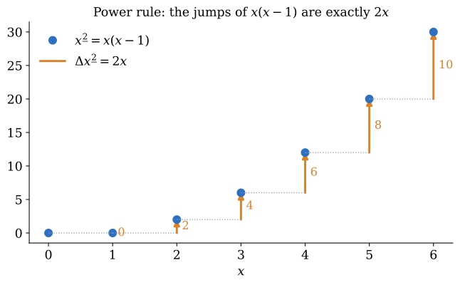
Where we can divide by \( n! \), as over \( \mathbb{Z} \) and \( \mathbb{Q} \), this is the rule for binomial coefficients, \( \Delta \binom{x}{n+1} = \binom{x}{n} \): this is Pascal's rule, and Newton's starting point. The differences also give Newton's series (shift_eq_sum_fwdDiff_iter, in Mathlib): for every function \( f \),
\[ f(x + n h) = \sum_{k=0}^{n} \binom{n}{k} , \Delta_h^{k} f(x) \]
exactly, with no remainder term. A polynomial of degree \( d \) has \( \Delta^{d+1} f = 0 \), so its Newton series stops after \( d + 1 \) terms. This is the finite version of Taylor's theorem, and here it's an identity rather than an approximation.
The fundamental theorem of calculus
Theorem (sum_fwdDiff). For every function \( f \), point \( x \), step \( h \), and number of steps \( n \),
\[ \sum_{k=0}^{n-1} \Delta_h f(x + k h) = f(x + n h) - f(x) \]
Proof. Write the sum out:
\[ \left( f(x + h) - f(x) \right) + \left( f(x + 2h) - f(x + h) \right) + \dots + \left( f(x + nh) - f(x + (n-1)h) \right) \]
Every middle value appears once with \( + \) and once with \( - \), so it cancels. Only the last value and the first value survive. \( \square \)
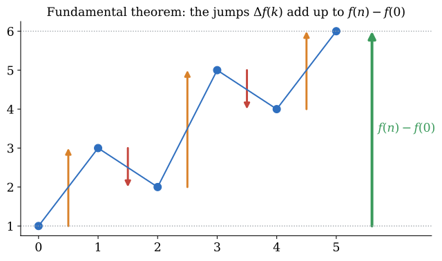
In the continuous theory, the fundamental theorem needs the completeness of \( \mathbb{R} \) and a limit on each side. Here it's a sum that telescopes, and it's exact for every function, not only the "nice" ones.
The product rule
Theorem (fwdDiff_mul). For all functions \( f \) and \( g \),
\[ \Delta_h (f g)(x) = f(x) , \Delta_h g(x) + \Delta_h f(x) , g(x + h) \]
Proof. Add and subtract \( f(x) , g(x + h) \):
\[ f(x+h) g(x+h) - f(x) g(x) = f(x) \left( g(x+h) - g(x) \right) + \left( f(x+h) - f(x) \right) g(x+h) \]
\( \square \)
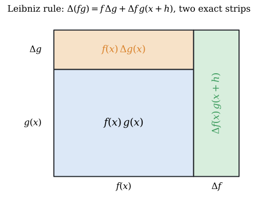
The picture explains the shifted \( g(x + h) \). When the rectangle grows, the strip on the right has the new height. In the continuous theory, the small corner where the two strips overlap is thrown away in the limit. Here nothing is thrown away: the corner belongs to the right strip, and the rule is exact.
The finite line \( \mathbb{Z}/p \)
The same calculus works on the finite line \( \mathbb{Z}/p \), the circle of \( p \) points where \( p - 1 \) is followed by \( 0 \), with values in \( \mathbb{F}_p \) or any level \( \mathbb{CT}_{k,p} \) of its Constructible tower. Something new happens there.
Theorem (fwdDiff_iter_char). If \( p \) is a prime and \( p = 0 \) among the values, then for every function \( f \),
\[ \Delta_h^{p} f(x) = f(x + p h) - f(x) \]
Proof, step by step:
- Applying \( \Delta_h \) \( p \) times gives the alternating binomial sum \( \Delta_h^{p} f(x) = \sum_{k=0}^{p} (-1)^{p-k} \binom{p}{k} f(x + k h) \).
- For \( 0 < k < p \), the prime \( p \) divides \( \binom{p}{k} = \frac{p!}{k! , (p-k)!} \), because it divides the numerator and not the denominator. Since \( p = 0 \) among the values, these terms vanish.
- Only \( k = p \) and \( k = 0 \) remain: \( f(x + p h) + (-1)^{p} f(x) \). For odd \( p \), \( (-1)^{p} = -1 \). For \( p = 2 \), \( +1 = -1 \) because \( 2 = 0 \). \( \square \)
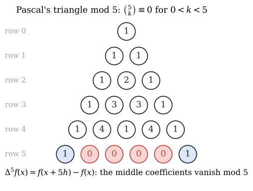
Corollary (fwdDiff_iter_zmod). On the finite line \( \mathbb{Z}/p \) with step \( 1 \), \( x + p = x \), so \( \Delta^{p} f = 0 \) for every function \( f \). The same is true on every level of the tower and for every step, as we'll see in the section on spaces with no edges.
So on a finite line, every function behaves like a polynomial of degree less than \( p \): its \( p \)-th difference vanishes. That's no accident. Every function \( \mathbb{F}_p \to \mathbb{F}_p \) is a polynomial of degree less than \( p \), and Newton's series writes it down.
The chain rule, and its restrictions
The chain rule is where finite calculus needs the most care, so let's go slowly.
Take \( F = f \circ g \), that is, \( F(x) = f(g(x)) \). Its difference is
\[ \Delta_h F(x) = f(g(x + h)) - f(g(x)) = f(g(x) + k) - f(g(x)), \qquad k = g(x + h) - g(x) = \Delta_h g(x) \]
So the difference of \( f \circ g \) is a difference of \( f \), at the point \( g(x) \), but with the step \( k = \Delta_h g(x) \) instead of \( h \). That one observation explains everything.
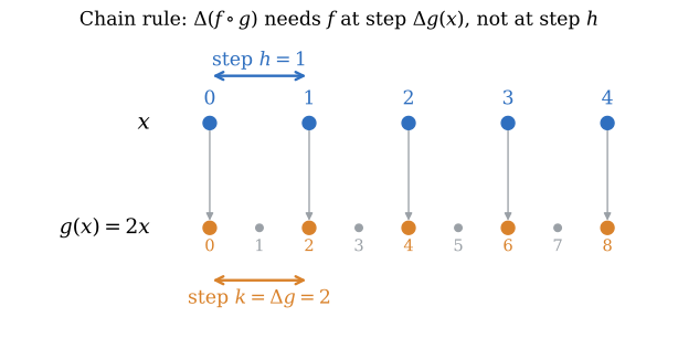
Restriction 1: the step changes from point to point. In the continuous theory, the derivative of \( f \) doesn't depend on a step, so \( (f \circ g)' = f'(g) \cdot g' \) can use \( f' \) directly. Here, the differences of \( f \) we know are at step \( h \), and the chain rule needs them at the step \( \Delta_h g(x) \), which in general is different at every \( x \). With the fixed step, the chain rule is simply false.
Theorem (chain_rule_fails). With \( f(x) = x^{2} \), \( g(x) = 2x \), and \( h = 1 \) on \( \mathbb{Z} \): \( \Delta (f \circ g)(0) = 4 \), but \( \Delta f(g(0)) \cdot \Delta g(0) = 1 \cdot 2 = 2 \).
Restriction 2: dividing by the step needs a field and a nonzero step. If we divide each difference by its own step, the chain rule holds exactly. The divided difference of \( f \) between \( a \) and \( b \) is \( f[a, b] = \frac{f(b) - f(a)}{b - a} \).
Theorem (chain_rule_divided). In any field, if \( h \neq 0 \) and \( g(x + h) \neq g(x) \), then
\[ (f \circ g)[x, x + h] = f[g(x), g(x + h)] \cdot g[x, x + h] \]
Proof. Multiply and divide by \( k = g(x + h) - g(x) \), which is allowed because \( k \neq 0 \) in a field. \( \square \)
So this version of the chain rule needs a field, which excludes \( \mathbb{Z} \), and it needs \( g \) to actually move: if \( g(x + h) = g(x) \), the outer divided difference is \( \frac{0}{0} \).
A notation that makes the chain rule ordinary. On the tower every level is a field, so we can always divide by a nonzero step. Define the difference quotient, with the step written in the denominator as Leibniz did:
\[ \frac{dF}{dh}(x) = \frac{\Delta_h F(x)}{h} = \frac{F(x + h) - F(x)}{h} \]
Theorem (dq_chain). For all functions \( f \) and \( g \) on a field, every point \( x \), and every step \( h \neq 0 \),
\[ \frac{d(f \circ g)}{dh}(x) = \frac{df}{dk}\left( g(x) \right) \cdot \frac{dg}{dh}(x), \qquad k = \Delta_h g(x) = h , \frac{dg}{dh}(x) \]
Proof. If \( k \neq 0 \), this is \( \frac{\Delta (f \circ g)}{h} = \frac{\Delta (f \circ g)}{k} \cdot \frac{k}{h} \), a cancellation of fractions, since \( f(g(x) + k) = f(g(x + h)) \). If \( k = 0 \), then \( g(x + h) = g(x) \), so the left side is \( 0 \), and the right side has the factor \( \frac{dg}{dh}(x) = 0 \). \( \square \)
This is the ordinary chain rule \( \frac{df}{dx} = \frac{df}{du} \cdot \frac{du}{dx} \), read literally: \( du \) is the actual increment of \( u = g(x) \), and the fractions cancel. In this notation the first two restrictions aren't obstacles any more, they are just what the symbols say: the derivative carries its step, and the outer step is the increment of the inner function. The condition that \( g \) moves isn't even needed. The fundamental theorem reads \( \sum_{k < n} h , \frac{dF}{dh}(x + kh) = F(x + nh) - F(x) \) (sum_dq), a Riemann sum that is exact.
What the notation can't remove is that the step is part of the derivative. In the continuous theory \( \frac{df}{dk} \) has the same limit for every \( k \), so the step can be forgotten. Here \( \frac{df}{dk} \) and \( \frac{df}{dh} \) are different functions.
Restriction 3: maps must send steps to steps. Differential forms, below, are built on a chosen set of steps. For a coordinate change \( g \) to carry forms from one chart to another, it must send the steps of the first chart to the steps of the second. This is the class of maps we'll use for charts below. It includes the rotations of the tower, as long as each chart carries its own steps.
There's a second finite calculus that does have an exact chain rule: the formal derivative of polynomials57, defined by the rule \( D(x^{n}) = n x^{n-1} \) and extended by linearity. It satisfies the power, product, and chain rules over every commutative ring (formal_rules), with no limit anywhere. But it only applies to polynomials, it has no fundamental theorem, and in characteristic \( p \) it has a surprise: \( D(x^{p}) = p x^{p-1} = 0 \) (derivative_X_pow_char), so a nonconstant function can have zero derivative. The two calculi split the classical one between them:
| Differences \( \Delta_h \) | Formal derivative \( D \) | |
|---|---|---|
| Applies to | every function, with a chosen step | polynomials |
| Power rule | for falling powers | for ordinary powers |
| Product rule | with a shift | exact |
| Chain rule | exact in Leibniz form \( \frac{d(f \circ g)}{dh} = \frac{df}{dk} \frac{dg}{dh} \), with \( k = \Delta_h g \) | exact, with no step |
| Fundamental theorem | exact | none |
| Stokes' theorem | exact, below | none |
| Charts allowed | maps that send steps to steps | every polynomial map, including rotations |
| Jacobian determinant | invisible to counting | exact, multiplicative |
The continuous calculus has every row at once, and the price is the limit.
Several variables
In a space with several chosen steps \( e_1, \dots, e_n \), for instance the unit steps of \( (\mathbb{CT}_{k,p})^{n} \), one in each direction, we have \( n \) partial differences \( \Delta_i f(x) = f(x + e_i) - f(x) \).
Theorem (fwdDiff_comm). Partial differences commute: \( \Delta_i \Delta_j f = \Delta_j \Delta_i f \).
Proof. Both sides equal \( f(x + e_i + e_j) - f(x + e_i) - f(x + e_j) + f(x) \), because \( x + e_i + e_j = x + e_j + e_i \). \( \square \)
In the continuous theory this is Schwarz's theorem on mixed partial derivatives, and it needs the second derivatives to be continuous. Here it holds for every function, because addition is commutative.
Differential forms on a frame of steps
Differential forms are the language of the general Stokes' theorem. With chosen steps, they're simpler than in the continuous theory, because a form is just a table of numbers58.
Fix a space \( M \) whose points can be added, such as \( (\mathbb{CT}_{k,p})^{n} \), and choose a frame: a list of steps \( e_1, \dots, e_n \) in \( M \). The steps can be any elements. The unit steps are one choice, \( \sqrt{3} , e_1 \) is another, and a frame may have more steps than \( M \) has coordinates. The frame cuts the space into cubes. A cube is a base point \( x \) together with a set \( T \) of directions: the cube at \( x \) spanned by the steps \( e_i \), \( i \in T \). When \( T \) has \( k \) directions, it's a \( k \)-cube. A \( 0 \)-cube is a point, a \( 1 \)-cube is an edge, a \( 2 \)-cube is a square, and so on. A \( k \)-form \( \omega \) assigns a number \( \omega(x, T) \) to every \( k \)-cube.
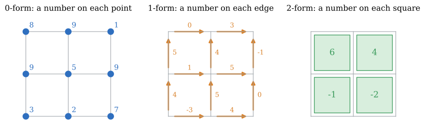
The exterior derivative \( d \) turns a \( k \)-form into a \( (k+1) \)-form:
\[ d\omega(x, T) = \sum_{i \in T} \sigma(T, i) , \Delta_i , \omega(\cdot, T \setminus \{i\})(x), \qquad \sigma(T, i) = (-1)^{\#\{ j \in T \ : \ j < i \}} \]
In words: for each direction \( i \) of the cube, take the difference across the cube in direction \( i \) of the face values that don't use \( i \), and add these up with alternating signs. The signs record the orientation. In the plane, this gives the familiar operators:
- For a \( 0 \)-form \( f \), \( df(x, \{i\}) = \Delta_i f(x) \): the gradient, one difference per edge.
- For a \( 1 \)-form with values \( P \) on horizontal edges and \( Q \) on vertical edges, \( d\omega(x, \{1, 2\}) = \Delta_1 Q(x) - \Delta_2 P(x) \): the curl, one number per square.
Why \( d \circ d = 0 \)
Theorem (d_d). For every form \( \omega \), in every dimension, \( d(d\omega) = 0 \).
In the plane this says that the curl of a gradient is zero, and in space also that the divergence of a curl is zero. Here is the proof, step by step:
- Expand twice. \( d(d\omega)(x, T) \) is a double sum over ordered pairs of distinct directions \( (i, j) \) in \( T \): first remove \( i \), then \( j \). Each term is \( \sigma(T, i) , \sigma(T \setminus \{i\}, j) , \Delta_i \Delta_j , \omega(\cdot, T \setminus \{i, j\})(x) \).
- Pair each term \( (i, j) \) with the term \( (j, i) \). Both use the same face \( T \setminus \{i, j\} \), and since partial differences commute, the same difference \( \Delta_i \Delta_j = \Delta_j \Delta_i \).
- Compare their signs. Say \( i < j \). Removing \( i \) first lowers by one the count of directions below \( j \), so \( \sigma(T \setminus \{i\}, j) = -\sigma(T, j) \). Removing \( j \) first doesn't change the count below \( i \), so \( \sigma(T \setminus \{j\}, i) = \sigma(T, i) \). The two signs are opposite.
- So the terms cancel in pairs, and the sum is \( 0 \). \( \square \)
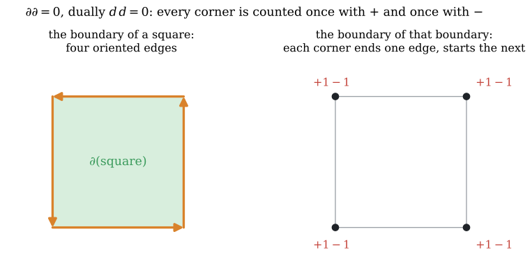
The picture shows the same fact from the side of the cubes. The boundary of a square is four oriented edges. The boundary of that boundary is the corners, and each corner appears twice: once as the end of an edge, with \( + \), and once as the start of the next edge, with \( - \). So the boundary of a boundary is zero, \( \partial \partial = 0 \), and \( d d = 0 \) is the same statement read through the forms.
Stokes' theorem
To integrate, we need regions. A chain \( c \) is a finite list of cubes with integer, or ring, coefficients, like "this square twice, minus that square". The integral of a form over a chain is the weighted sum of its values:
\[ \int_c \omega = \sum_{(x, T)} c(x, T) , \omega(x, T) \]
The boundary of a cube is the signed list of its faces:
\[ \partial (x, T) = \sum_{i \in T} \sigma(T, i) \left( (x + e_i, \ T \setminus \{i\}) - (x, \ T \setminus \{i\}) \right) \]
that is, for each direction \( i \), the far face minus the near face. The boundary of a chain is the sum of the boundaries of its cubes, with their coefficients.
Theorem (stokes). For every chain \( c \) and every form \( \omega \), in every dimension and every degree,
\[ \int_{\partial c} \omega = \int_c d\omega \]
Proof, step by step:
- Both sides are linear in \( c \): the integral of a sum of chains is the sum of the integrals. So it's enough to prove it for a single cube \( c = (x, T) \).
- For a single cube, the left side is \( \sum_{i \in T} \sigma(T, i) \left( \omega(x + e_i, T \setminus \{i\}) - \omega(x, T \setminus \{i\}) \right) \).
- That is \( \sum_{i \in T} \sigma(T, i) , \Delta_i , \omega(\cdot, T \setminus \{i\})(x) \), which is exactly the definition of \( d\omega(x, T) \). \( \square \)
So with a frame of steps, Stokes' theorem is almost a definition: \( d \) is built to be the exact counterpart of \( \partial \). Its content shows when \( c \) is a large region. Then the faces shared by two neighbouring cubes appear twice, with opposite orientations, and cancel. Only the outer boundary survives.
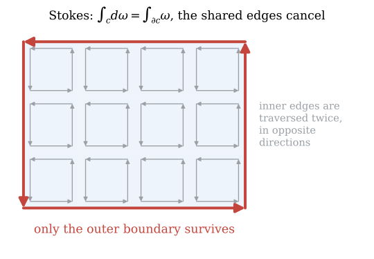
For a rectangle of \( m \times n \) unit squares in the integer grid \( \mathbb{Z}^{2} \), the first-level picture, this is Green's theorem (green):
\[ \sum_{a < m} \sum_{b < n} \left( \Delta_1 Q - \Delta_2 P \right)(a, b) = \sum_{a < m} P(a, 0) + \sum_{b < n} Q(m, b) - \sum_{a < m} P(a, n) - \sum_{b < n} Q(0, b) \]
The left side adds the curl over the squares. The right side goes around the boundary counterclockwise: along the bottom, up the right side, back along the top, down the left side. And in one dimension, a chain of \( n \) consecutive edges has the two endpoints as its boundary, which is the fundamental theorem of calculus from before.
A space with no edges
Now the finite world shows an advantage. On the torus \( (\mathbb{Z}/N)^{n} \), modular arithmetic glues each side to the opposite side: after \( N - 1 \) comes \( 0 \) again. The "reset" from \( N - 1 \) to \( 0 \) is not an edge. It's the seam where the square is glued into a closed surface, like a video game screen where leaving on the right brings you back on the left.
Theorem (sum_d_eq_zero). On the torus, or on any finite group, for every form \( \omega \) and every shape \( T \), the sum of \( d\omega \) over all cubes is zero:
\[ \sum_{x} d\omega(x, T) = 0 \]
Proof, step by step:
- Expand \( d\omega \) and exchange the two sums. It's enough to show that \( \sum_x \Delta_i , \omega(\cdot, T')(x) = \sum_x \omega(x + e_i, T') - \sum_x \omega(x, T') \) is zero, for each direction \( i \).
- The shift \( x \mapsto x + e_i \) is a bijection of the torus: it moves every point one step and wraps the last one around to the first. So \( \sum_x \omega(x + e_i, T') \) adds the same values as \( \sum_x \omega(x, T') \), in a different order.
- The two sums are equal, and their difference is zero. \( \square \)
This is Stokes' theorem on a closed space: the torus has no boundary, so the integral of every \( d\omega \) over all of it vanishes. The proof only used that the space is finite and that points can be added, so it holds on every \( (\mathbb{CT}_{k,p})^{n} \), for every frame. Every level of the tower is closed in this sense, in every direction: \( p \) steps of any size \( h \), even \( h = \sqrt{3} \), come back to the start, because \( p \cdot h = 0 \). So on every level, and for every step, \( \Delta_h^{p} f = 0 \) for every function (fwdDiff_iter_level). In the continuous theory, the closed torus has to be built as a quotient of \( \mathbb{R}^{2} \). Here it's simply what modular arithmetic already is.
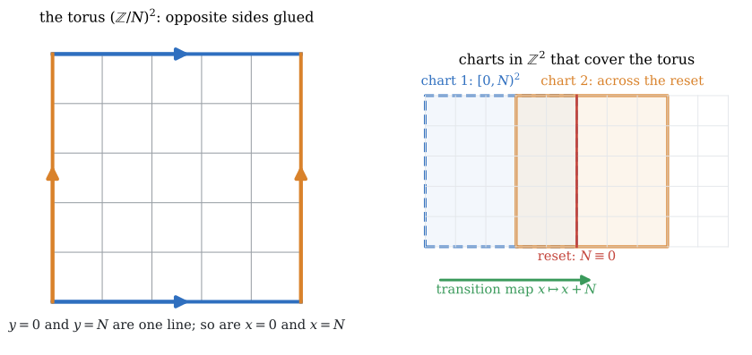
Charts, transition maps, and pullbacks
On a manifold we compute in local coordinates, called charts, and move between overlapping charts by transition maps. The finite torus works the same way, and the reset is exactly where we'd want a second chart. We start with the integer grid, which for \( N = p \) is the first level \( \mathbb{F}_p \) in every coordinate, and then state the theorems for any space and any frame, which covers every level.
A chart is a patch of the infinite grid \( \mathbb{Z}^{n} \), mapped onto the torus by the reduction
\[ \pi : \mathbb{Z}^{n} \to (\mathbb{Z}/N)^{n}, \qquad \pi(x_1, \dots, x_n) = (x_1 \bmod N, \dots, x_n \bmod N) \]
One chart is the box \( [0, N)^{n} \). Its points near \( N - 1 \) are on the seam, so a second chart is a box that straddles the seam, such as \( [N - 2, 2N - 2) \times [0, N) \). On the overlap, the two charts describe the same torus points by coordinates that differ by \( N \), and the transition map is the translation \( x \mapsto x + N e_1 \).
What kind of map can we use? By restriction 3 of the chain rule, it must send steps to steps. Call \( \varphi \) a step map if
\[ \varphi(x + e_i) = \varphi(x) + e'_i \quad \text{for every point } x \text{ and direction } i \]
so that \( \varphi \) carries each cube to a cube of the same shape. The pullback of a form \( \omega \) along \( \varphi \) reads \( \omega \) in the new coordinates: \( (\varphi^{\ast}\omega)(x, T) = \omega(\varphi(x), T) \).
Theorem (isStepMap_add_right, isStepMap_toTorus). Translations are step maps, and so is the reduction \( \pi \). So all our charts and transition maps are step maps.
Proof. For a translation, \( (x + e_i) + c = (x + c) + e_i \). For the reduction, \( \pi \) respects addition, and it sends the unit step \( e_i \) of \( \mathbb{Z}^{n} \) to the unit step \( e_i \) of the torus. \( \square \)
Theorem (d_pullback). For every step map \( \varphi \) and every form \( \omega \), \( d(\varphi^{\ast}\omega) = \varphi^{\ast}(d\omega) \).
Proof. Each term of \( d(\varphi^{\ast}\omega)(x, T) \) contains \( \omega(\varphi(x + e_i), \dots) - \omega(\varphi(x), \dots) \). Since \( \varphi(x + e_i) = \varphi(x) + e'_i \), this is \( \omega(\varphi(x) + e'_i, \dots) - \omega(\varphi(x), \dots) \), which is the corresponding term of \( d\omega(\varphi(x), T) \). \( \square \)
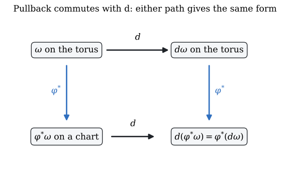
This is what makes charts useful. To compute \( d\omega \) near the seam, pull \( \omega \) back to the chart that straddles the seam, compute there with ordinary integer coordinates, and the result is the pullback of the true \( d\omega \). Different charts agree, because pullbacks compose:
Theorem (pullback_comp). \( (\psi \circ \varphi)^{\ast} = \varphi^{\ast} \circ \psi^{\ast} \).
So pulling back to one chart and then across a transition map is the same as pulling back to the other chart directly. Integrals transform correctly too. If \( \varphi_{\ast} c \) is the chain \( c \) moved forward along \( \varphi \), cube by cube:
Theorem (integral_pushforward, bd_pushforward). The change of variables formula \( \int_{\varphi_{\ast} c} \omega = \int_c \varphi^{\ast}\omega \) holds, and for a step map, moving a chain commutes with taking its boundary: \( \partial(\varphi_{\ast} c) = \varphi_{\ast}(\partial c) \).
Finally, a form on the torus, read in a chart, repeats with period \( N \) in every direction (toTorus_periodic): \( (\pi^{\ast}\omega)(x + N e_i, T) = (\pi^{\ast}\omega)(x, T) \). That's the reset seen from the chart: \( N \) steps in any direction bring us back to the same point of the torus.
Rotations, the volume form, and the Jacobian
So far the charts were patches of the integer grid. On the Constructible tower we don't need the integer grid at all. The space \( (\mathbb{CT}_{k,p})^{n} \) is itself a finite group, so by the theorem on spaces with no edges it's already closed: every direction wraps around, like the torus. The reduction \( \pi \) isn't needed, and a chart is simply a map from \( (\mathbb{CT}_{k,p})^{n} \) to \( (\mathbb{CT}_{k,p})^{n} \). This makes room for rotations.
Rotations exist in every finite field. The rational circle of this post works in any field. For every \( t \) with \( 1 + t^{2} \neq 0 \),
\[ c = \frac{1 - t^{2}}{1 + t^{2}}, \qquad s = \frac{2t}{1 + t^{2}}, \qquad c^{2} + s^{2} = 1 \]
(rot_circle), and the rotation \( (x, y) \mapsto (c x - s y, \ s x + c y) \) preserves \( x^{2} + y^{2} \) (rotation_preserves_norm). Over \( \mathbb{F}_7 \) the circle \( c^{2} + s^{2} = 1 \) has exactly \( 8 \) points (circle_count_7): seven from \( t \in \mathbb{F}_7 \), since \( -1 \) has no square root there, and one more, \( (-1, 0) \), from \( t = \infty \). So the plane \( \mathbb{F}_7^{,2} \) has exactly \( 8 \) rotations. These are the multiplications by the \( 8 \) elements of norm \( 1 \) in \( \mathbb{F}_7(i) \), from the section on the new symbols.
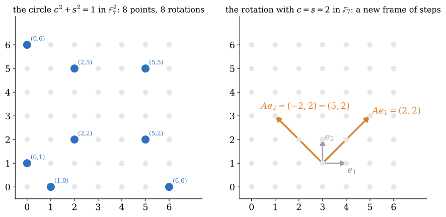
Rotations in the difference calculus need their own frame. A rotation \( A \) sends the unit steps \( e_1, e_2 \) to new steps \( A e_1, A e_2 \). It is a step map from the frame \( (e_1, e_2) \) onto the frame \( (A e_1, A e_2) \) (isStepMap_frame), so every theorem of the previous section applies: pullback commutes with \( d \), and change of variables and Stokes hold, as long as each chart carries its own frame of steps. What doesn't hold is that the two frames give the same calculus. Over \( \mathbb{F}_7 \), \( (2, 2) \) is a rotation of \( (1, 0) \), since \( 2^{2} + 2^{2} = 8 = 1 \). For \( f(x, y) = xy \),
\[ \Delta_{(2,2)} f(0, 0) = 4, \qquad \text{but} \qquad 2 , \Delta_1 f(0, 0) + 2 , \Delta_2 f(0, 0) = 0 \]
(rotated_frame_differs). A difference along a rotated step isn't the rotated combination of the unit differences. This is the first restriction of the chain rule again: differences remember the step.
Why a frame-free calculus can't act on functions. The continuous derivative has an exact product rule, \( D(fg) = f , Dg + g , Df \), with no shift. On a finite space, that rule alone forces the derivative to vanish.
Theorem (derivation_finite_eq_zero). On the functions on a finite set, every linear map \( D \) with the exact product rule is zero.
Proof, step by step:
- Let \( e \) be the indicator of one point: \( 1 \) there, \( 0 \) elsewhere. Then \( e \cdot e = e \).
- The product rule gives \( D e = D(e \cdot e) = 2 e , D e \).
- Multiplying by \( e \) gives \( e , D e = 2 e , D e \), because \( e \cdot e = e \). So \( e , D e = 0 \), and by step 2, \( D e = 0 \).
- Every function is a finite sum of point indicators times constants, \( f = \sum_x f(x) , e_x \). So \( D f = \sum_x f(x) , D e_x = 0 \). \( \square \)
So an exact product rule, and with it an exact chain rule, can't live on the functions of a finite space. It lives on polynomials, the finite formulas, before we evaluate them. This is the formal calculus of the earlier table, and on the Constructible tower it does everything the difference calculus can't.
The chain rule, exact in every dimension. For a polynomial map \( \varphi = (\varphi_1, \dots, \varphi_m) \) and a polynomial \( f \),
\[ \partial_i (f \circ \varphi) = \sum_{j} (\partial_j f \circ \varphi) \cdot \partial_i \varphi_j \]
(chain_rule). Proof: by building \( f \) up from constants, sums, and products with a variable. For a constant both sides are \( 0 \). Both sides are additive. And for \( f \cdot x_k \), the product rule on the left matches the product rule on the right, term by term. \( \square \)
The Jacobian. Collect the partial derivatives into the Jacobian matrix \( J\varphi \), whose entry in row \( j \) and column \( i \) is \( \partial_i \varphi_j \). The chain rule says exactly that the Jacobian of a composite is the product of the Jacobians, \( J(\psi \circ \varphi) = (J\psi \circ \varphi) \cdot J\varphi \) (jac_comp), and since the determinant of a product is the product of the determinants,
\[ \det J(\psi \circ \varphi) = (\det J\psi \circ \varphi) \cdot \det J\varphi \]
(det_jac_comp), in every dimension.
The volume form. In the plane, a \( 1 \)-form is \( P , dx + Q , dy \), a \( 2 \)-form is \( g , dx \wedge dy \), and \( d(P , dx + Q , dy) = (\partial_x Q - \partial_y P) , dx \wedge dy \). The pullback substitutes \( \varphi \): \( \varphi^{\ast} dx = d\varphi_1 \) and \( \varphi^{\ast} dy = d\varphi_2 \). The volume form \( dx \wedge dy \) then pulls back to
\[ \varphi^{\ast} dx \wedge \varphi^{\ast} dy = \det J\varphi \cdot dx \wedge dy \]
(volume_pullback). Proof: \( \varphi^{\ast} dx \wedge \varphi^{\ast} dy = (\partial_x \varphi_1 , dx + \partial_y \varphi_1 , dy) \wedge (\partial_x \varphi_2 , dx + \partial_y \varphi_2 , dy) \). Since \( dx \wedge dx = dy \wedge dy = 0 \) and \( dy \wedge dx = -dx \wedge dy \), only \( \partial_x \varphi_1 \partial_y \varphi_2 - \partial_y \varphi_1 \partial_x \varphi_2 = \det J\varphi \) remains. \( \square \)
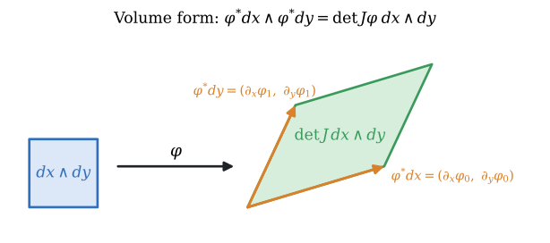
With the pullback of \( 2 \)-forms defined this way, \( \varphi^{\ast}(g , dx \wedge dy) = (g \circ \varphi) \det J\varphi , dx \wedge dy \), the exterior derivative commutes with every polynomial pullback: \( d(\varphi^{\ast} f) = \varphi^{\ast}(df) \) for functions (d0_pullback, the chain rule) and \( d(\varphi^{\ast}\omega) = \varphi^{\ast}(d\omega) \) for \( 1 \)-forms (d1_pullback). In the proof of the second, the second derivatives of \( \varphi \) cancel because \( \partial_x \partial_y = \partial_y \partial_x \), and the rest is the determinant. A rotation has \( J = \begin{pmatrix} c & -s \\ s & c \end{pmatrix} \), so \( \det J = c^{2} + s^{2} = 1 \) (rotation_det): rotations preserve the volume form, in every finite field.
Where the Jacobian goes when we count. On a finite space, the honest integral of a function is the sum of its values over all points. That sum doesn't change under any bijection of the space (sum_comp_equiv), because it just adds the same numbers in another order. So counting never sees a Jacobian factor: a map with \( \det J = 4 \), like \( (x, y) \mapsto (2x, 2y) \) on \( \mathbb{F}_7^{,2} \), permutes the points, and the count stays the same. And counting gives the formal derivative no fundamental theorem: over \( \mathbb{F}_3 \), \( D(x^{5}) = 5x^{4} \), and \( \sum_{x \in \mathbb{F}_3} 5x^{4} = 1 \neq 0 \) (formal_ftc_fails), while the difference calculus gives exactly \( 0 \) on a closed space.
So on the Constructible tower, calculus comes in two exact halves. The difference calculus has the fundamental theorem and Stokes' theorem for counting integrals, and allows charts that carry their own frames. The formal calculus has the exact product and chain rules, all polynomial charts including rotations, and the Jacobian determinant with the volume form. In the continuous theory, the limit glues the two halves into one.
What this calculus doesn't do yet
Three honest limits:
- One calculus for both halves. The difference calculus has Stokes' theorem, and the formal calculus has the Jacobian. No single finite calculus has both, and the theorem on derivations shows why it can't act on functions with an exact product rule.
- Forms of every degree in every dimension, in the formal calculus. The chain rule and the multiplicativity of the Jacobian determinant are proved in every dimension, but the pullback of forms commuting with \( d \) is proved here in the plane only.
- Faces of a box. Stokes' theorem holds for every chain, but the statement that the boundary of a full box of cubes is exactly its outer faces is proved here only in dimensions \( 1 \) and \( 2 \), as the fundamental theorem and Green's theorem.
Still, the result is striking. Derivatives, the fundamental theorem, the product rule, several variables, differential forms with \( d \circ d = 0 \), Stokes' theorem, closed spaces without boundary, charts, transition maps, pullbacks, and change of variables all exist as exact, finite statements, over every finite world of this post, and none of them needs a limit or a completed infinity. What the limit buys, in the continuous theory, is to have all the rules of the table at once: the exact chain rule and the fundamental theorem, for all smooth coordinate changes. Each is still available here, one finite calculus at a time.
Patches with different primes
The charts of the calculus section overlap only on strips near their edges. Nothing then forces one prime on the whole space: each patch may carry its own. This section asks what keeps differences and integrals consistent where two such patches meet, and how the answer depends on the curvature of the space. Every theorem is proved in Lean4, in the file Patches.lean.
A whole patch can't be glued, a strip can
Take a patch \( U \) with values in \( \mathbb{F}_p \), a patch \( V \) with values in \( \mathbb{F}_q \), and \( p \neq q \). If a step map carried all of \( U \) into \( V \), going \( p \) steps around \( U \) would come back to the start, so the image step \( e' \) would satisfy \( p , e' = 0 \) in \( \mathbb{F}_q \). Since \( p \) is invertible modulo \( q \), \( e' = 0 \): every step is squashed to nothing (whole_patch_squashed).
But on a manifold the overlap is only a strip, much narrower than \( p \), and nothing ever wraps around there. To carry a value from \( U \) to \( V \), read it as the integer of smallest size, between \( -\frac{p}{2} \) and \( \frac{p}{2} \), and reduce that integer modulo \( q \). This transfer isn't additive on all of \( \mathbb{F}_p \), since nothing additive is. But it is exact inside the window of small numbers (transfer_intCast), and it respects a sum or a product whenever the result doesn't overflow (transfer_add, transfer_mul).
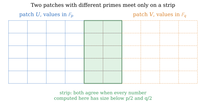
Theorem (strip_fwdDiff, strip_sum). Let the data on the strip be integers of size at most \( H \). Then:
- a \( k \)-th difference computed in \( U \) and carried to \( V \) is the \( k \)-th difference computed in \( V \), as soon as \( 2 \cdot 2^{k} H < p \);
- a sum of \( w \) values along the strip carries over exactly, as soon as \( 2 w H < p \).
Proof, step by step:
- Reducing integers modulo \( p \) respects \( + \) and \( - \), so a difference computed in \( U \) is the reduction of the same difference computed with integers (
fwdDiff_iter_cast). The same holds in \( V \). - Each difference at most doubles the size, so the \( k \)-th difference has size at most \( 2^{k} H \) (
abs_fwdDiff_iter_le). A sum of \( w \) values has size at most \( w H \). - These integers lie inside the window of \( p \), where the transfer reads them back exactly. \( \square \)
So the condition for consistency on a strip is
\[ \min(p, q) > 2 \times \text{the largest number the calculus on the strip produces} \]
It doesn't tie \( p \) to \( q \). Each prime only has to exceed the size of what is computed on the strip, and two very different primes can be glued as long as both are large enough.
The sphere on its equatorial strip
The sphere needs two charts, the stereographic projections from the north pole and from the south pole. The transition between them is the inversion \( z \mapsto \frac{1}{\bar{z}} \), that is
\[ (x, y) \mapsto \left( \frac{x}{x^{2} + y^{2}}, \ \frac{y}{x^{2} + y^{2}} \right) \]
which is its own inverse in every field (inv2_inv2). Each chart's window covers the region around its own pole. Moving away from it, the coordinates grow until they leave the window, and that is exactly where the other chart takes over. So in a finite chart, leaving the window is what marks the chart's edge. The two windows meet on a strip around the equator.
Theorem (sphere_strip). Let \( z = \frac{a + b i}{c} \) be a point with integers \( |a|, |b|, |c| \le H \), \( c \neq 0 \), \( z \neq 0 \), and let \( 2 H^{2} < p \). Then in \( \mathbb{F}_p \) the inversion of \( z \) is defined, it equals the reduction of the rational point \( \frac{(c a, \ c b)}{a^{2} + b^{2}} \), and the numerators and the denominator of that point have size at most \( 2 H^{2} \).
Proof. The integers \( c \) and \( a^{2} + b^{2} \) are nonzero and smaller than \( p \), so they're nonzero modulo \( p \). The formula is then an identity of fractions, valid in every field (inv2_frac), and the bounds are \( |c a| \le H^{2} \) and \( a^{2} + b^{2} \le 2 H^{2} \). \( \square \)
Both patches compute the reduction of the same rational point, so they agree. And the result can be read back unambiguously: fractions with numerators and denominators of size at most \( K \) that agree modulo \( p \) are equal as rationals once \( 2 K^{2} < p \) (strip_readable). With \( K = 2H^{2} \), that's \( 8 H^{4} < p \), for both primes.
On the whole patch, consistency is impossible. For \( p \equiv 3 \pmod 4 \), the sphere over \( \mathbb{F}_p \) has \( p^{2} + 1 \) points, and over \( \mathbb{F}_q \) it has \( q^{2} + 1 \), so there isn't even a one-to-one correspondence. What's more interesting is which differences a strip can't see. Whether the sphere is "plane plus one point" depends on \( p \bmod 4 \), through the question of whether \( x^{2} + y^{2} = 0 \) has a nonzero solution. On the whole patch it does exactly when \( p \not\equiv 3 \pmod 4 \) (isotropic_iff). Inside the window it never does, for any \( p \): a sum of two small squares, not both zero, lies strictly between \( 0 \) and \( p \) (window_anisotropic). So no strip can detect \( p \bmod 4 \). It behaves like topology: a property of the whole space that no local patch sees. Matching the primes modulo \( 4 \) is a condition for matching the global shapes, not for local consistency.
Outside the window, the strip breaks down. Over \( \mathbb{F}_5 \), the point \( 1 + 2i \), of size \( 2 \), has \( 1^{2} + 2^{2} = 5 = 0 \), so its inversion isn't even defined (inversion_undefined_F5). That's no contradiction: \( 2 \cdot 2^{2} = 8 \) isn't below \( 5 \), so this point is outside the window of \( \mathbb{F}_5 \).
Curvature decides how large the primes must be
The torus of the calculus section has translations as transitions, and the sphere has the inversion. The first is linear, the second isn't. That difference isn't a choice of charts. It's forced by curvature, and it changes how large the primes must be. There are two steps.
Step 1: curvature forces curved vertices. Take a closed surface made of squares, like the surface of a cube: every square has \( 4 \) corners and \( 4 \) sides, and every edge is a side of exactly \( 2 \) squares. Around a vertex lying on \( \deg v \) squares, the angles add up to \( \deg v \) quarter turns. A full turn is \( 4 \), so the angle defect at \( v \) is \( 4 - \deg v \) quarter turns. It's the discrete curvature at \( v \), as in Descartes' theorem on polyhedra59.
Theorem (gauss_bonnet). On every closed square surface, with \( V \) vertices, \( E \) edges, and \( F \) squares,
\[ \sum_{v} \left( 4 - \deg v \right) = 4 \chi, \qquad \chi = V - E + F \]
that is, the total defect is \( 2\pi \chi \). This is the discrete Gauss–Bonnet theorem60.
Proof, step by step:
- Count the corners of the squares in two ways. By vertex, there are \( \sum_v \deg v \). By square, there are \( 4F \).
- Count the pairs (edge, square containing it) in two ways. By square, there are \( 4F \). By edge, there are \( 2E \). So \( E = 2F \).
- Then \( \sum_v (4 - \deg v) = 4V - 4F = 4(V - 2F + F) = 4(V - E + F) \). \( \square \)
A step-map chart around a vertex is a patch of the square grid, and in the grid every vertex lies on \( 4 \) squares. So a step-map chart can exist only at a flat vertex, one with \( \deg v = 4 \). Two consequences:
- If every vertex is flat, then \( \chi = 0 \) (
flat_euler_zero). Only a surface with \( \chi = 0 \), like the torus, can be covered by step-map charts alone. - If every vertex lies on at least \( 3 \) squares, at least \( 4 \chi \) vertices are curved (
curved_vertices). On the cube, \( \chi = 8 - 12 + 6 = 2 \), and all \( 8 \) corners are curved, each with a defect of one quarter turn (cube_curvature).
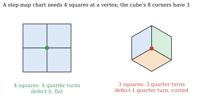
At a curved vertex no step-map chart exists, so the transition there can't be a step map, and it can't be linear. This is the finite counterpart of Benzécri's theorem61: a closed surface has an atlas of affine charts only if \( \chi = 0 \).
Step 2: the price of a transition, in the size of the primes. A linear transition keeps sizes linear. An affine map with integer entries of size at most \( a \) and shifts of size at most \( N \) sends data of size at most \( H \) in \( n \) dimensions to data of size at most \( n a H + N \) (affine_window). For a translation of the torus the matrix is the identity, and the bound is simply \( H + N \). So on a flat space the strips need
\[ p, \ q > 2 \left( n a H + N \right) \]
which grows linearly with the data. The inversion squares sizes. In \( n \) dimensions it is \( x \mapsto \frac{c , x}{x_1^{2} + \dots + x_n^{2}} \), and its numbers reach \( H^{2} \) and \( n H^{2} \) (inversion_window). This growth is forced, not an artifact of the bound: the strip point \( H + (H - 1) i \), of size \( H \), is sent to a point whose first coordinate has reduced denominator \( H^{2} + (H - 1)^{2} \ge H^{2} \) (inversion_growth_sharp). So on the sphere the window must at least contain \( H^{2} \), and \( 8 H^{4} < p \) is enough to read the results back. The dimension enters as the factor \( n \).
Put together: curvature, through \( \chi \neq 0 \), forces vertices where no step-map chart exists. There the transitions are nonlinear. For the sphere the transition is the inversion, whose strips need primes that grow like a power of the data, while flat transitions need primes that grow only linearly. The primes on overlapping patches don't constrain each other. The curvature decides how large each must be compared with the data on the strips, and the class of the primes, like \( p \bmod 4 \) for the sphere, carries the global shape.
One step is still missing. Lean proves the quadratic cost for the inversion, the transition the sphere actually uses. It doesn't prove that every nonlinear transition costs as much. For polynomial and rational maps of degree \( d \) this is a classical fact about heights38: sizes grow like \( H^{d} \). But it isn't formalized here.
Levels against iterations
In \( \mathbb{R} \), and in constructive analysis as well, a number like \( \sqrt{2} \) is reached by an iteration. Newton's rule \( x \mapsto \frac{1}{2}\left( x + \frac{2}{x} \right) \), started at \( 1 \), gives
\[ 1, \quad \frac{3}{2}, \quad \frac{17}{12}, \quad \frac{577}{408}, \quad \dots \]
whose squares miss \( 2 \) by \( 1 \), \( \frac{1}{4} \), \( \frac{1}{144} \), \( \frac{1}{166464} \), and so on. The misses shrink, but the iteration never ends, and no term of it squares to \( 2 \).
In the Constructible tower a number is reached by a level. In \( \mathbb{CT}_5 \), \( 2 \) is not a square in \( \mathbb{F}_5 \), so one level adds the symbol \( \sqrt{2} \), and \( \left( \sqrt{2} \right)^{2} = 2 \) holds exactly (sqrt_two_new_F5). In \( \mathbb{CT}_7 \) not even that is needed: \( 3^{2} = 9 = 2 \), so \( \sqrt{2} = 3 \) is already at level \( 0 \) (sqrt_two_examples). After that the construction is over.
The same holds for every radical, not only square roots. Whenever a number \( d \) of some level has no \( n \)-th root there, the next level adds one, as a placeholder symbol \( \alpha \) with the single rule \( \alpha^{n} = d \), and from then on \( d^{\frac{1}{n}} \) is an exact number of the tower (exists_root_next_level, proved for every level, every \( d \), and every \( n \)). Over \( \mathbb{F}_7 \), for example, \( \sqrt[3]{1} = 1 \) and \( \sqrt[3]{6} = 3 \) are already there, since \( 3^{3} = 27 = 6 \). The other cube roots are new, by the rule of the section on new symbols. A single level \( \mathbb{F}_7(\alpha) \), with \( \alpha^{3} = 2 \) and \( 343 \) elements \( a + b\alpha + c\alpha^{2} \), holds all of them at once (cube_roots_F343):
\[ \sqrt[3]{2} = \alpha, \qquad \sqrt[3]{3} = 3\alpha^{2}, \qquad \sqrt[3]{4} = \alpha^{2}, \qquad \sqrt[3]{5} = 3\alpha \]
Each is exact: for instance \( \left( 3\alpha^{2} \right)^{3} = 27 \alpha^{6} = 27 \cdot 4 = 108 = 3 \) in \( \mathbb{F}_7 \). In \( \mathbb{R} \), each of these four numbers is again an iteration that never ends.
This is the difference between the two number systems, and here is what it buys.
| Iterations in \( \mathbb{R} \) | Levels in \( \mathbb{CT}_p \) | |
|---|---|---|
| \( \sqrt{2} \), \( \sqrt[3]{2} \), \( \sqrt[3]{3} \), or any root of a polynomial | a sequence that never ends | a finished object after finitely many levels |
| The defining equation, like \( x^{2} = 2 \) | never holds for any term | holds exactly |
| How much work is needed | depends on the precision asked, without end | known in advance: a polynomial of degree \( d \) has all its roots by a level of degree dividing \( \mathrm{lcm}(1, \dots, d) \) |
| \( +, -, \times, \div \) | on approximations, with errors that grow | exact, and each one terminates |
| Are two numbers equal? | can't be decided in general | a finite computation |
| Memory for one number | unbounded | fixed: \( N_k \) digits modulo \( p \) at a level of degree \( N_k \) |
| All roots of all polynomials | needs completeness, or one new kind of symbol per polynomial | radicals alone, in fact single roots of unity |
| The conjugate and the inverse | computed on approximations | a power \( z \mapsto z^{q} \), and a finite formula |
| The whole space | can't be listed or counted | finite at each level: it can be listed, counted, and summed over |
| Integration | a limit of sums, for well-behaved functions only | a finite sum, for every function |
| Fundamental theorem, mixed partial differences, Stokes | need continuity or differentiability | exact for every function |
| A closed space, like the torus | a quotient of \( \mathbb{R}^{n} \) | what the arithmetic already is |
| Proof by checking every case | impossible | possible, and used by the Lean proofs of this post |
| Probability of a single point | zero, yet the point can happen | \( \frac{1}{\text{number of points}} \), never zero |
| Order and position | built into the numbers | exact inside a window of small numbers; beyond it, defined by a chosen metric |
Three of these rows deserve a comment.
Ruler and compass, in finite levels. Every length that ruler and compass construct is reached from the rationals by finitely many square roots. The same recipe can be followed in \( \mathbb{CT}_p \), for every prime \( p \) that divides none of the denominators involved, and there each square root costs one level at most, and nothing if the root is already present. So everything ruler and compass construct, and by the same argument everything origami constructs, has an exact counterpart at a finite level of the tower. By the fundamental theorem of the tower, the same holds for every root of every polynomial.
The paradox of zero probability. My previous post2 started from this paradox: on the real line, choosing one point has probability zero, yet some point is always chosen. At a level of the tower the paradox can't be stated. The space is finite, every point has the probability \( \frac{1}{\text{number of points}} \), and these probabilities add up to \( 1 \).
Proof by checking every case. Because a level is finite, a statement about all of its numbers can be proved by trying them all. Several theorems of this post were proved that way, by the Lean kernel running through every element of a level with \( 49 \) or \( 2401 \) numbers.
What about order?
The iterations do answer one question that a level doesn't. The terms \( 1, \frac{3}{2}, \frac{17}{12}, \dots \) tell us that \( \sqrt{2} \) lies between \( 1.41 \) and \( 1.42 \): where it sits among the rationals. The tower has no order that respects its arithmetic. No finite field can, since adding \( 1 \) to itself \( p \) times comes back to \( 0 \), while in an ordered field \( 1 + 1 + \dots + 1 > 0 \) (no_compatible_order). So this isn't a choice we could undo by a cleverer definition: no order of the usual kind exists on any level. Does that make \( \mathbb{CT}_p \) weaker than \( \mathbb{R} \)? I don't think so, for three reasons.
The numbers we write down keep their order. When \( p \) is huge, everything we actually write is far from the point where the arithmetic wraps around. Integers of size at most \( H \) stay distinct modulo \( p \) as soon as \( p > 2H \) (small_int_injective), and fractions \( \frac{a}{b} \) with \( |a|, |b| \le H \) stay distinct as soon as \( p > 2H^{2} \) (small_rat_injective). And as long as a sum or a product stays below \( p \), it is the integer sum or product, with no wrap-around (small_integers_exact). So inside this window the bounded rationals of this post live in \( \mathbb{F}_p \) exactly, with their sums, their products, and their usual order. Nothing that a measurement has ever produced is outside such a window.
The place of \( \sqrt{2} \) was never given by the algebra. Algebra can't tell \( \sqrt{2} \) from \( -\sqrt{2} \): both satisfy \( x^{2} = 2 \). In the number system \( \mathbb{Q}(\sqrt{2}) \), whose numbers are \( a + b\sqrt{2} \), conjugation \( a + b\sqrt{2} \mapsto a - b\sqrt{2} \) respects every sum and product, fixes every rational, and swaps \( \sqrt{2} \) with \( -\sqrt{2} \) (conj_swaps_roots). So every property that arithmetic can express holds for \( \sqrt{2} \) exactly when it holds for \( -\sqrt{2} \), and \( \mathbb{Q}(\sqrt{2}) \) carries two orders, mirror images of each other: one with \( \sqrt{2} > 0 \), one with \( \sqrt{2} < 0 \). In \( \mathbb{R} \) the order can be defined from arithmetic alone, \( x \ge 0 \) exactly when \( x \) is a square, but only because every positive real number has a square root, which is the completeness of \( \mathbb{R} \) again. In \( \mathbb{Q}(\sqrt{2}) \) the same rule decides nothing, since neither \( \sqrt{2} \) nor \( -\sqrt{2} \) is a square there (sqrt_two_sign_undecided). What places \( \sqrt{2} \) at \( 1.414\dots \) is the order of \( \mathbb{R} \), a separate structure. In the tower that structure isn't forced on us. Among the residues, \( \sqrt{2} \) is \( 3 \) or \( 4 \) for \( p = 7 \), \( 6 \) or \( 11 \) for \( p = 17 \), \( 5 \) or \( 18 \) for \( p = 23 \), \( 8 \) or \( 23 \) for \( p = 31 \) (sqrt_two_positions). It isn't lined up with the integers at all, and it doesn't have to be.
Distance is a structure we choose, in geometry too. Euclidean geometry ties distance to the order of the number line. Geometry since Riemann doesn't: a space gets its distances from a metric, a structure put on it, and the coordinates carry no distance of their own. The tower fits this view well. A metric there is a symmetric matrix \( G \), and the squared length of a vector \( v \) is \( v \cdot G v \), an exact number of the tower. The Euclidean metric \( x^{2} + y^{2} \) is one choice among many. Every map \( A \) with \( A^{\mathsf{T}} G A = G \) preserves every squared length exactly (isometry_preserves), as the rotations did for \( x^{2} + y^{2} \). Where \( \sqrt{2} \) lies relative to other numbers is then a consequence of the metric we define, not a fact about the number.
Even the constructions don't fix the order. The straightedge only joins points and intersects lines, and that needs no metric: of three points on a line, which one lies between the other two is the same for every metric. The compass is different. A circle is the set of points at one distance from its center, so drawing a circle reads the metric. An origami fold reads it too, since a fold is a reflection, and a reflection needs to know what is perpendicular. Now follow the recipe for \( \sqrt{2} \): draw the unit square, open the compass to its diagonal, and carry the diagonal to the first axis. With the metric \( x^{2} + a y^{2} \), the diagonal \( (1, 1) \) has squared length \( 1 + a \), and a point \( (x, 0) \) on the axis has squared length \( x^{2} \). So the compass lands at the point \( x \) with \( x^{2} = 1 + a \) (diagonal_on_axis):
| Metric | Where the recipe lands | Its place among the rationals |
|---|---|---|
| \( x^{2} + y^{2} \) | \( \sqrt{2} \) | between \( 1.41 \) and \( 1.42 \) |
| \( x^{2} + 2y^{2} \) | \( \sqrt{3} \) | between \( 1.73 \) and \( 1.74 \) |
| \( x^{2} + 3y^{2} \) | \( 2 \) | exactly on a rational |
The same steps, with the same ruler and compass, land between \( 1.41 \) and \( 1.42 \) under one metric and exactly on \( 2 \) under another. So the place of a constructed number among the rationals isn't produced by the construction. It is read off the metric we chose, and the Euclidean one is one choice among many.
So can order be defined concretely? Yes, but only after a choice. In any number system we actually construct, an order comes from choosing a metric, or from choosing which root plays the role of the positive one. Once chosen, it can be defined exactly. What doesn't exist is an order that the construction itself hands us.
So order isn't lost so much as moved: from something built into the numbers to something we define on top of them, for the range of numbers and the geometry at hand. That is already how it works for every constructed number system, as the last two paragraphs show. \( \mathbb{R} \) hides the choice inside its completeness, and the tower makes it explicit. What I can't offer yet is the finished theory of such metrics. Comparing two distances, saying which is larger, still needs an order on the values, and beyond the window that order has to be defined, not found. That work is open.
With this, my claim is that \( \mathbb{CT}_p \) is the stronger number system. \( \mathbb{R} \) gives the position of a number through an iteration that never ends. \( \mathbb{CT}_p \) gives the number itself, exactly, in finitely many levels, and leaves position to the metric.
Conclusion
The first half of this post argued that all the objections share one move: start from a finite rule with no stopping condition, then speak about its never-finished unfolding as if it were a finished object. The successor function becomes "the set of all natural numbers". Lattice refinement becomes "the continuum of points in a cube". A digit-generating program becomes "the number \( \pi \) with its infinitely many digits". And "we don't know a bound" becomes "there is no bound in the world". Infinity is a property of rules. As a claim about objects, it has never been constructed, never been observed, and has to be assumed by an axiom precisely because it can't be shown.
The second half paid the debt this leaves. The Constructible tower \( \mathbb{CT}_p \) is built from the integers modulo a prime by adding one new symbol per level, each with a finite multiplication rule. A formula says which symbols are new. The first of them, for half of the primes, is \( i = \sqrt{-1} \), and all the others have the same kind of algebra, with a conjugation and a norm. Whatever root a level misses, a later level adds, so the tower has its own fundamental theorem of algebra, without the completeness of \( \mathbb{R} \). And calculus lives on every level of it: differences with an exact fundamental theorem, the chain rule in Leibniz's form, differential forms with Stokes' theorem, spaces without boundary, charts, rotations, and the Jacobian. Different patches of a space don't even need the same prime: on the strips where they overlap, they agree as soon as both primes exceed the size of the data there, and curvature decides how fast that size grows.
Against the iterations of \( \mathbb{R} \), this is my claim: \( \mathbb{CT}_p \) is the stronger number system, because it gives each number exactly, in finitely many levels, where \( \mathbb{R} \) gives only an approach that never ends. It has no order built in. But the small numbers we write down keep their order, and for the rest, position is a matter of the metric we put on a space, as it has been in geometry since Riemann.
Some things are still open, and it's better to say so. Constructive analysis is another constructive payment of the debt, and this post doesn't refute it. The theory of metrics on the tower, and of comparing distances beyond the window of small numbers, isn't written yet. The finite calculus comes in two halves, differences and formal derivatives, that the limit glues together in the continuous theory. That every nonlinear transition between patches costs as much as the sphere's inversion is a classical fact about heights, not yet formalized here. And which primes, and how many levels, a physical theory would need, and whether one prime for the whole space or one per patch, is a question for experiment, exactly as the principles of this post demand.
Until someone shows me the infinite set they chose from, invention remains construction, and math remains invention. The Constructible tower is one more invention, with the advantage that it can actually be built.
References
Generated with code: a cube refined into finer and finer finite lattices, the successor chain \( S^{k}(0) \), and the digits of \( \pi \) fading out where the computation stops.
Stephen Schanuel, Heights in number fields, Bulletin de la Société Mathématique de France 107 (1979), 433–449
Cite
If you found this work useful, please consider citing:
@misc{hadilq2026Constructible,
    author = {{Hadi Lashkari Ghouchani}},
    note = {Published electronically at \url{https://hadilq.com/posts/the-constructible-tower/}},
    gitlab = {Gitlab source at \href{https://gitlab.com/hadilq/hadilq.gitlab.io/-/blob/main/content/posts/2026-11-18-the-constructible-tower/index.md}},
    title = {The Constructible tower},
    year={2026},
}