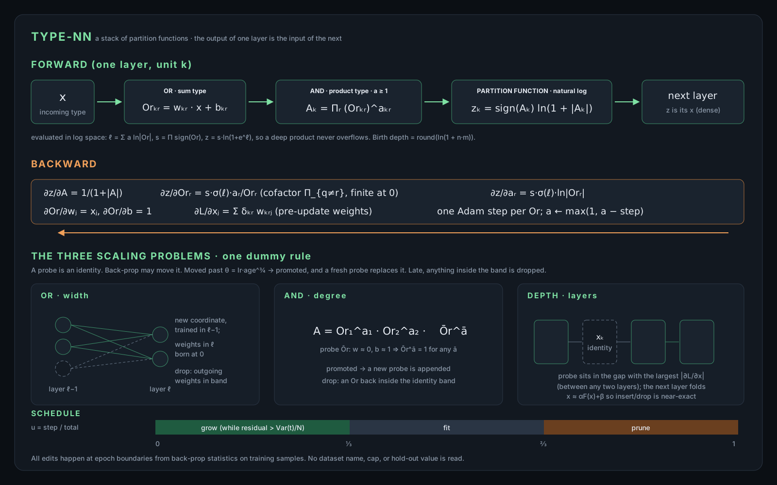
In the Type Mechanics¹ post we said something that sounded like a side remark: you organize knowledge by factorizing parent nodes out of the bulk of Type Generating Functions, TGFs. Well, it was not a side remark! If that sentence is true, then knowledge is a structure made of sum-types and product-types, and a structure like that can be trained. That's the whole idea of this post.

We will build a neural network whose layers are nothing but partition functions, where each partition function is a TGF evaluated on the data. Then we will let the back propagation not only move the numbers inside those TGFs, but also add and remove the types themselves: new alternatives (\(or\)), new conditions (\(and\)), and new levels of abstraction (depth). The result is called type-nn. In the end we compare it honestly with an ordinary MLP, and look at what it gets right and what it doesn't, yet.

The same notice as always! A path to perfection is zig-zag, so this is not a perfect version. Mistakes are expected, some of them intentionally, to increase the fun. The code, the benchmark and the Coq proofs are all in the repository², so you can count your points faster than before.

Let's dive in!

Knowledge is a tree of types

Let's remember what we built in the Type Mechanics¹. A type is a property we assign to objects, and its TGF counts the objects with that type. The sum-type is the \(or\) and its TGF is the sum of TGFs. The product-type is the \(and\) and its TGF is the product of TGFs.

\[ \eta(A+B)=\eta(A)\oplus\eta(B), \qquad \eta(A\times B)=\eta(A)\otimes\eta(B) \]

We also said the atomic types are not promised to be concrete. If our knowledge increases, we find new classifications, and the old atomic types are rewritten as sums and products of new ones. And we said a theory of a domain is what you get when you factorize the bulk TGF of that domain, since the factored-out terms are exactly the common properties, the abstractions, the parent nodes of the tree.

So knowledge has three moving parts:

1. which alternatives exist on a node, the \(or\)s,
2. which conditions must hold together, the \(and\)s,
3. how many levels of abstraction sit between the raw observations and the conclusion, the depth of the tree.

Keep these three in mind, since they will come back as the three scaling problems.

Partition functions are generating functions

In Statistical Mechanics³ the partition function is

\[ Z(\beta)=\sum_{s} e^{-\beta E_s} \]

which is a generating function in disguise: it counts states, weighted by \(e^{-\beta E}\), and every thermodynamic quantity is a derivative of \(\ln Z\). The logarithm is not decoration. Counting is multiplicative, since independent systems multiply their numbers of states, but information is additive, so the Boltzmann entropy is \(S=k\ln W\)⁴. A product-type of two independent types has \(n\times m\) objects, and \(\ln(nm)=\ln n+\ln m\) is the amount of knowledge it takes to pick one of them.

Now take a data point \(x\) with \(n\) coordinates. An \(or\) over those coordinates, with some counting weights, is a sum-type evaluated at \(x\):

\[ Or_{k,r}(x)=w_{k,r}\cdot x+b_{k,r} \]

An \(and\) of such \(or\)s is a product-type evaluated at \(x\):

\[ A_k(x)=\prod_r Or_{k,r}(x)^{a_{k,r}} \]

Here \(a_{k,r}\) is the assembly index from the Assembly theory⁵: how many times the sub-object \(Or_{k,r}\) is used to assemble \(A_k\). Raising a factor to \(a\) is literally \(a\) copies of the same type in the product. In the Assembly theory the number of reuses is what separates something assembled from something random, so it deserves to be a first-class parameter.

\(A_k\) is a partition function of the data point: a count of the ways \(x\) can be explained by pairing one alternative from each \(or\). Take its logarithm to turn the count into knowledge:

\[ z_k=\operatorname{sign}(A_k)\ln\left(1+|A_k|\right) \]

The \(1+\) makes the empty type carry zero knowledge, \(\ln 1=0\). The sign keeps the debt! Remember that in the Counting space a negative coefficient means the number of objects is in debt, counted by an observer that starts counting in the future. The logarithm acts on the size of the count, and the sign carries the debt through.

So a layer is a vector of partition functions, and its output \(z\) is the knowledge the layer extracted from \(x\), measured in nats.

A hierarchy of partition functions

What if that knowledge is itself the data for the next level? Then the next layer builds \(or\)s and \(and\)s over \(z\) instead of \(x\):

\[ x \xrightarrow{\ \text{layer }1\ } z^{(1)} \xrightarrow{\ \text{layer }2\ } z^{(2)} \longrightarrow \cdots \longrightarrow y \]

This is a generating function of generating functions, the same move as substitution in Analytic combinatorics⁶, where you plug one TGF into another to count structures made of structures. Each level counts the ways the previous level's knowledge can be combined.

Here is the claim of this post.

Claim

The hierarchy of partition functions, with its \(or\)s, \(and\)s and assembly indices, is our knowledge of the data. Its parent nodes are the factored-out abstractions, and its depth is the number of abstraction levels between observation and conclusion.

It's a claim, not a theorem, since "knowledge" is not a formal object here. But the structure is exactly the tree from the Type Mechanics, with two differences. First, it is dense: every \(or\) may read every coordinate of the level below, so it's a graph, and a tree only after pruning. Second, the counting weights are real numbers, so a coefficient can be in debt, and can be fractional.

If the claim is right, then training this hierarchy is training our knowledge, and the structure of the trained hierarchy is something we can reason about with \(and\) and \(or\).

Training the numbers

The numbers are the easy part, since back propagation⁷ already knows how to do it. We only need the Jacobians, and they are small and pretty.

Let \(g=\partial L/\partial z_k\). The logarithm contributes

\[ \frac{\partial z}{\partial A}=\frac{1}{1+|A|} \]

which is even, positive, and never larger than one. So the partition function can only compress knowledge; it never amplifies a gradient. The product contributes the cofactor, the product of all the other factors:

\[ \frac{\partial A}{\partial Or_r}=a_r\,|Or_r|^{a_r-1}\prod_{q\neq r}Or_q^{a_q} \]

and the assembly index gets its own gradient,

\[ \frac{\partial z}{\partial a_r}=\frac{\partial z}{\partial A}\,A\ln|Or_r| \]

The \(or\)s are linear, so \(\partial Or/\partial w_j=x_j\) and \(\partial Or/\partial x_j=w_j\). That's all of back propagation for this architecture.

In the computer we never form the product \(A\), since a deep product overflows. We keep \(\ell=\sum_r a_r\ln|Or_r|\) and the sign \(s\), and use

\[ z=s\ln\left(1+e^{\ell}\right), \qquad \frac{\partial z}{\partial Or_r}=s\,\sigma(\ell)\,\frac{a_r}{Or_r} \]

where \(\sigma\) is the logistic function. It's the same Jacobian, written so it never divides by zero where it matters.

Theorem 1

The log-space formulas are the partition function and its Jacobian: \(F(s e^\ell)=s\ln(1+e^\ell)\) and \(F'(A)\,A=s\,\sigma(\ell)\), where \(F(A)=\operatorname{sign}(A)\ln(1+|A|)\). Moreover \(F'(A)=1/(1+|A|)\) is a real derivative for \(A\neq 0\), and \(|F(A)|\le|A|\).

Proof

For \(s=\pm1\), \(|s e^\ell|=e^\ell\), and the rest is algebra. The derivative follows by composing \(\ln\) with \(1\pm x\) on each side of zero, and \(|F(A)|\le|A|\) is \(\ln(1+u)<u\), which is \(1+u<e^u\) in disguise. The machine-checked version is in the Coq development² as F_log_space, log_space_slope, F_deriv_pos, F_deriv_neg and F_abs_le.

Training the types

Now the interesting part. If knowledge has three moving parts, then training knowledge has three scaling problems.

1. \(or\) scaling: a new alternative. The level below discovers a new coordinate, a new atomic type, and the level above can start using it.
2. \(and\) scaling: a new condition. A product gets one more factor.
3. Depth scaling: a new level of abstraction, a new parent node inserted between two existing levels.

All three are solved with one rule, which I call the dummy rule. A new type is born as an identity, a type that changes nothing. Back propagation is free to move it. If back propagation moves it out of the identity, the type has earned its place, and a new dummy is born to keep probing. Late in training, anything that went back to the identity is dropped.

What is an identity for each operator? That's where the algebra of types pays off.

• For an \(and\), the identity is the unit type, the factor \(1\): \(w=0,\ b=1\), and \(1^{a}=1\) for any assembly index.
• For an \(or\), the identity is the empty contribution, the term \(0\): a new coordinate enters every \(or\) of the next level with weight \(0\).
• For depth, the identity is a level whose unit \(k\) is just \(x_k\), one \(or\) that copies one coordinate.

Theorem 2

Adding an identity \(or\) to an \(and\), or adding a coordinate to a level while the next level meets it with zero weights, does not change what the network computes.

Proof

The first is \(A\cdot 1^{a}=A\). For the second, \(b+\sum_j w_j x_j+0\cdot x_{new}=b+\sum_j w_j x_j\), whatever \(x_{new}\) is. So the new coordinate can be trained freely in the level below while the level above has not noticed it yet. In Coq these are and_probe_exact and width_probe_net.

For depth the story is more subtle, and I like it more for that reason. The identity level has \(A_k=x_k\), but then the partition function makes \(z_k=\operatorname{sign}(x_k)\ln(1+|x_k|)\), which is \(x_k\) only to first order. A new level of abstraction is never free: it compresses what passes through it. So when we insert it, the next level absorbs the best affine correction \(x\approx\alpha F(x)+\beta\) measured on the data, and the insertion is as close to exact as the compression allows. It's exact whenever the correction is exact, which is fold_exact in Coq. I find this a nice statement about knowledge in general: a new abstraction always costs a little, and the level above has to recalibrate to it. Remember the Calibration section of the Type Mechanics¹? It's the same ladder.

Where do we put a new level? Between any two levels, not only at the ends. The dummy level sits in the gap where \(|\partial L/\partial x|\) is largest, the gap where the knowledge is most sensitive, and moves there again every epoch until it is promoted.

When did back propagation move it?

This is the question that decides everything, and it is harder than it looks. The optimizer is Adam⁸, and Adam normalizes its steps. A parameter that receives pure noise still moves, like a random walk, about \(\eta\sqrt{T}\) after \(T\) steps. A parameter that receives a gradient with a consistent sign moves up to \(\eta T\). So "it moved" must mean "it moved more than noise would move it". The decision boundary is at the geometric mean of the two scales:

\[ \theta(T)=\sqrt{\eta\sqrt{T}\cdot\eta T}=\eta\,T^{3/4} \]

Theorem 3

For \(T\ge1\), \(\eta\sqrt T\le\theta(T)\le\eta T\), and noise/\(\theta\) = \(\theta\)/drift = \(T^{-1/4}\).

Proof

Monotonicity of \(T^{p}\) in \(p\) for \(T\ge1\), and \(T^{3/4}\cdot T^{3/4}=T^{1/2}\cdot T\). In Coq: threshold_between, threshold_geometric_mean, threshold_separates.

The ratio \(T^{-1/4}\) shrinks as the dummy ages, so noise falls behind the threshold and a real push catches up with it. No constant here was fitted to any data set; \(\eta\) is the learning rate and \(T\) is the age.

There was one more trap, and the first experiments walked right into it. Adam's steps don't know how small a gradient is, only how consistent it is. When the network had already fitted the training data to \(10^{-15}\), tiny but consistent gradients still pushed dummies around, and one run of XOR grew to 1,464 parameters. The dummies were promoted because the optimizer moved them, not because the data needed them! The fix comes from the data itself. The constant predictor, the model that knows nothing, has loss \(\operatorname{Var}(t)\). We grow only while the training residual is worth more than one sample's share of that,

\[ L_{\text{train}}>\frac{\operatorname{Var}(t)}{N} \]

since below that line the data has nothing left to pay for a new type. It's a nice rule for knowledge too: don't invent a new concept for less than one observation's worth of surprise.

Finally the schedule: grow in the first third of the training, fit in the second, prune in the last. Scaling up early and down late is what we do when we learn a subject, where first we collect every alternative that could matter, and then we forget the ones that went back to nothing.

The prior of knowledge

The dummy rule tells us when a new type may be born. It doesn't tell us whether the new type was worth it, and that matters. A type-nn that promotes on the dummy rule alone, which I kept as type-nn-overfit, keeps almost every type the back propagation touched, and fits its training data about ten times more tightly than an ordinary MLP, without predicting new data any better.

Knowledge shouldn't work like that! We don't rewrite our theory of a domain every time an observation moves it a little. We expect significant evidence before we change our prior. There is a classic way to say how significant: the Bayesian information criterion⁹. A type with \(k\) parameters, judged on \(n\) observations, is worth keeping only if

\[ n\ln\frac{\text{MSE}_{\text{without it}}}{\text{MSE}_{\text{with it}}} \;>\; k\ln n \]

Each parameter costs \(\ln n\) nats of prior, and the type has to buy them back with evidence. The nice part is how we measure "without it". We reset the type to its identity, \(1\) for an \(and\) factor and \(0\) for an \(or\) term, and look at the data again. So the question "is this type part of our knowledge?" becomes "does the data notice when we replace it with nothing?". And when the answer is no, dropping it is exact, since it is already the identity.

The same rule decides in both directions. A dummy is promoted only if it moved and it pays, and in the last third of the training the network forgets every type the data no longer pays for, as long as the whole model doesn't become a worse explanation than the best one it has had.

Reasoning with the trained knowledge

A trained type-nn is a graph of \(and\)s and \(or\)s with counting weights. You can read it.

Take XOR, the classic example. A single layer with one \(and\) can express it exactly: one \(or\) with assembly index two,

\[ A=c\,(x_0-x_1)^{2},\qquad c=e-1 \]

The sum-type \(x_0-x_1\) is \(\pm1\) when exactly one input is on and \(0\) otherwise. Assembling it twice erases the sign, and \(c=e-1\) makes the partition function land on \(z=\ln(1+c)=1\). Compare it with the TGF of \(xor\) in the Type Mechanics, which factored into \(-not\otimes(\langle+\lceil\oplus\langle-\lceil)\): there, too, \(xor\) was a product built on a sum. A product of sums is the only thing type-nn knows how to build, so this factorization is the kind of structure its growth is searching for. To be honest, the trained XOR networks in the benchmark are not this minimal yet. They grow to two or three levels, which is one more reason the pruning needs work.

This is the sense in which we can reason with a trained type-nn. Every live \(or\) is an alternative, every live \(and\) is a conjunction, every assembly index says how many times a sub-object was reused, and every level is one step of abstraction. Pruning removes what went back to identity, so what is left is the structure the data asked for. The logical graph is the knowledge.

What it buys over an MLP

Let's be concrete about what a trained knowledge graph gives us that an MLP doesn't, and what it costs. I'll mark each point by how strong the evidence is today: measured on the benchmark, structural when it follows from the architecture and is proved or tested but not yet shown on real data, and hypothesis when it's neither.

It's not a black box (structural). Every unit of type-nn is an explicit \(and\) of \(or\)s with assembly indices, and the same move that pruning uses, resetting a type to its identity, works on a trained network too. The reset is exact (Coq's and_probe_exact and drop_zero_column), and its effect on the loss can be measured, not guessed. So when the training data carries a bias, say a feature that stands in for something you don't want the model to use, you can find the factors that lean on it, set them to the identity, and retrain the rest. The same goes for any behaviour you don't want. An MLP unit is one weighted sum behind a ReLU; there is no factor to cut. To be fair, the weights inside an \(or\) are still dense real numbers, and I haven't yet shown such an edit removing a real bias from a real data set. That's an experiment worth doing next.

It chooses its own shape (measured). The width, the number of factors in each \(and\), and the depth are found during the training; an MLP needs its hidden width and depth picked by hand. The training knobs, the learning rate and the number of epochs, are still there for both, so it's the architecture hyper-parameters that disappear, not all of them.

It needs fewer parameters (measured). Five of six tasks, down to a ninth of the MLP on diabetes, while predicting clearly better on diabetes and ionosphere and indistinguishably on wine and wdbc.

It could make small local models (hypothesis). A model that grows only the structure its data pays for is exactly what you'd want on a laptop or a phone, local LLMs included. But nothing here tests that: every result is on small tabular data, and there's no sequence model, batching, or GPU path yet.

And the costs:

• it still needs more parameters than the MLP on iris;
• measuring evidence makes training slower, up to about 25 times the MLP on these tasks;
• on tiny networks a logarithm per factor makes inference slower, up to about 9 times;
• it still overfits the training set, because its prior measures noise by the training error itself;
• inserting a new level of abstraction is near-exact, not exact, since the logarithm forbids an exact identity layer.

Does it work?

Honesty first. On data sets this small, one random seed can make or break a comparison, so every number below is a mean over five seeds, and a win counts only when it's outside the noise. The audit of the benchmark is in the repository²; please read it, it is the most important file there.

The current benchmark treats every model the same way:

• the same split, standardized on the training rows only;
• the same shuffle, optimizer, loss, epochs and learning rate;
• the same readout \(F\);
• five seeds, with every learnable number counted.

The baseline, c-mlp, is a Linear–ReLU–Linear network with the same readout. type-nn-overfit promotes on the dummy rule alone and is kept frozen as a reference; type-nn is the one with the prior of knowledge.

task	type-nn	type-nn-overfit	c-mlp	params type-nn / overfit / c-mlp
iris	0.0215 ± 0.0069	0.0249 ± 0.0044	0.0280 ± 0.0061	125 / 175 / 67
wine	0.0277 ± 0.0048	0.0209 ± 0.0105	0.0234 ± 0.0056	170 / 393 / 275
wdbc	0.0448 ± 0.0048	0.0459 ± 0.0030	0.0438 ± 0.0017	163 / 163 / 513
diabetes	0.0329 ± 0.0010	0.0371 ± 0.0015	0.0488 ± 0.0042	20 / 33 / 193
ionosphere	0.0886 ± 0.0111	0.0813 ± 0.0119	0.1461 ± 0.0155	154 / 298 / 577

The numbers are hold-out mean squared errors. With the prior, type-nn needs fewer parameters than c-mlp on every task but iris, down to a ninth of them on diabetes, and it clearly predicts better on diabetes and ionosphere. On iris, wine and wdbc the differences are within the noise of five seeds, in both directions. So it's a real result, but not a sweep, and I'd rather tell you that than round it up.

It also shows what's still missing. The prior uses the training error as its measure of noise, and on these networks the training error is tiny, so the prior is most lenient exactly where the network overfits most. A better estimate of the noise, one that doesn't need to peek at the hold-out, is the next iteration. The schedule, the thirds, should become as dynamic as the threshold already is, too.

Conclusion

A partition function is a generating function evaluated on the data, and its logarithm is knowledge in nats. Stacking them gives a hierarchy of generating functions, the factorized tree of types we called a theory in the Type Mechanics. With type-nn, back propagation trains the counting weights of that tree, and the dummy rule trains its shape: new alternatives, new conditions, new levels of abstraction, each born as an identity, promoted when the data moves it, and kept only while the data pays for it.

So we can train our knowledge, and then reason about it with \(and\) and \(or\) on a graph. It isn't magic! It's the same boring, constructive algebra of counting, running on a computer.

---

Appendix: the equations of type-nn

Everything the implementation computes, in one place.

Forward. Layer \(\ell\) maps \(x\in\mathbb{R}^{n_\ell}\) to \(z\in\mathbb{R}^{m_\ell}\), and \(n_{\ell+1}=m_\ell\). Unit \(k\):

\[ Or_{k,r}=w_{k,r}\cdot x+b_{k,r},\qquad A_k=\prod_r Or_{k,r}^{a_{k,r}},\qquad z_k=\mathrm{sign}(A_k)\ln(1+|A_k|) \]

with \(o^{a}:=\mathrm{sign}(o)|o|^{a}\) and \(a_{k,r}\ge 1\). In log space,

\[ \ell_k=\sum_r a_{k,r}\ln|Or_{k,r}|,\qquad s_k=\prod_r \mathrm{sign}(Or_{k,r}),\qquad z_k=s_k\ln\left(1+e^{\ell_k}\right) \]

Birth. \(\mathrm{round}\left(\ln(1+nm)\right)\) layers, \(n\to m\to\cdots\to m\), one random \(or\) per unit.

Backward. With \(\sigma\) the logistic function,

\[ \frac{\partial z}{\partial A}=\frac{1}{1+|A|},\qquad \frac{\partial z}{\partial Or_r}=s\,\sigma(\ell)\,\frac{a_r}{Or_r},\qquad \frac{\partial z}{\partial a_r}=s\,\sigma(\ell)\ln|Or_r| \]

\[ \frac{\partial Or}{\partial w_j}=x_j,\qquad \frac{\partial Or}{\partial b}=1,\qquad \frac{\partial L}{\partial x_j}=\sum_{k,r}\delta_{k,r}\,w_{k,r,j},\qquad \delta_{k,r}=\frac{\partial L}{\partial z_k}\frac{\partial z_k}{\partial Or_{k,r}} \]

At \(Or_r=0\) exactly, \(\partial z/\partial Or_r\) is the cofactor \(\prod_{q\neq r}Or_q^{a_q}\) when \(a_r=1\) and \(0\) when \(a_r>1\); \(\partial z/\partial a_r=0\). The loss gradient is mean-MSE, \(\partial L/\partial y=(y-t)/m\).

Growth gate. Grow only while the epoch's training error is unexplained:

\[ \mathrm{MSE}_{\text{train}}>\frac{\mathrm{Var}(t)}{N},\qquad t=y-m\frac{\partial L}{\partial y} \]

Threshold. A probe of age \(T\) steps has moved when its RMS distance from the identity exceeds

\[ \theta(T)=\eta\,T^{3/4}=\sqrt{\eta\sqrt{T}\cdot\eta T} \]

type-nn-overfit also drops anything inside the band \(\theta(N)\).

Depth fold. Inserting an identity layer at a junction, the next layer absorbs \(x\approx\alpha F(x)+\beta\): \(w'_j=\alpha_j w_j\) and \(b'=b+\sum_j w_j\beta_j\). Removing one absorbs \(F(x)\approx\alpha' x+\beta'\) the same way.

Evidence (type-nn). With \(n=Nm\) training observations, an item with \(k\) parameters is kept, or promoted, only if

\[ n\ln\frac{\mathrm{MSE}_{\text{without}}}{\mathrm{MSE}_{\text{with}}}>k\ln n \]

where \(\mathrm{MSE}_{\text{without}}\) is measured with the item reset to its identity. Pruning keeps the model criterion \(C=n\ln\mathrm{MSE}+K\ln n\), with \(K\) the number of parameters, at or below its best value seen while pruning.

References

Cite

If you found this work useful, please consider citing:

@misc{hadilq2026TrainTheKnowledge,
    author = {{Hadi Lashkari Ghouchani}},
    note = {Published electronically at \url{https://hadilq.com/posts/train-the-knowledge/}},
    gitlab = {Gitlab source at \href{https://gitlab.com/hadilq/hadilq.gitlab.io/-/blob/main/content/posts/2026-09-22-train-the-knowledge/index.md}},
    title = {Train the knowledge},
    year={2026},
}